Visualization
the visualizations rely on CairoMakie.jl.
poles and zeros of a transfer function
g = (s + 2) / (s^2 + 1/4)
viz_poles_and_zeros(g)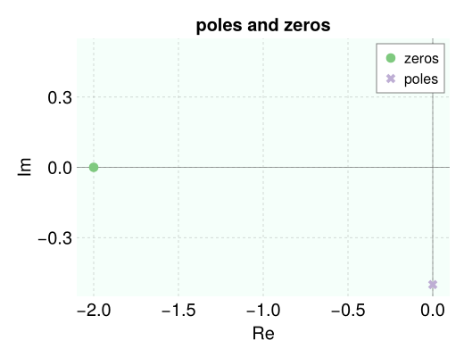
response of a system to an input
g = 4 / (4 * s ^ 2 + 0.8 * s + 1)
U = 1 / s
Y = g * U
data = simulate(Y, 50.0)
viz_response(data, title="SO underdamped step response")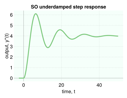
Nyquist diagram
g = 1 / (s^2 + s + 1)
nyquist_diagram(g)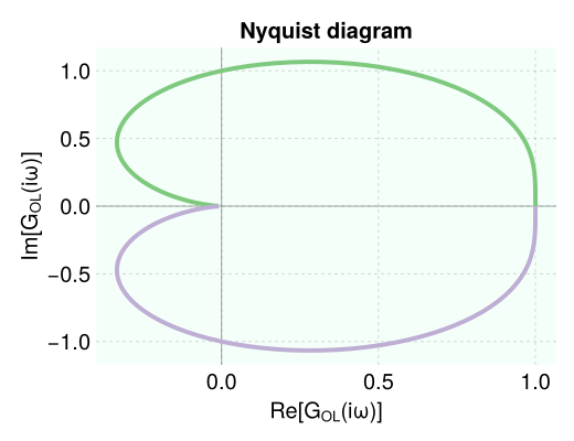
Bode plot
g = 3 / (s + 1)
bode_plot(g, log10_ω_min=-4.0, log10_ω_max=4.0, nb_pts=300)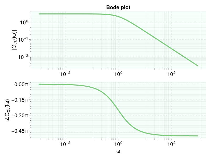
the range of frequencies presented is determined by log10_ω_min and log10_ω_max. the resolution of the Bode plot is determined by nb_pts.
see gain_phase_margins to compute the gain and phase margins and the critical and gain crossover frequencies.
Root locus plot
g_ol = 4 / (s + 3) / (s + 2) / (s + 1)
root_locus(g_ol)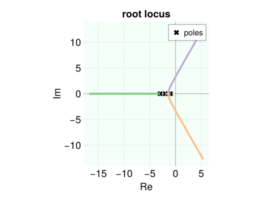
modifying the figures
all visualization functions return a Figure object from CairoMakie.jl that can be further modified. for example:
g_ol = 4 / (s + 3) / (s + 2) / (s + 1)
fig = root_locus(g_ol)
ax = current_axis(fig)
xlims!(ax, -15, 5)
ax.xlabel = "real numbers"
cool plot theme
the custom plot theme can be invoked in CairoMakie.jl for other plots via:
using Controlz, CairoMakie
set_theme!(cool_theme)
more, CairoMakie.jl offers other themes here.
detailed docs
Controlz.viz_response — Functionviz_response(data,
title="", xlabel="time, t",
ylabel="output, y*(t)",
savename=nothing)plot data[:, :output] vs. data[:, :t] to visualize the response of a system to an input. typically the data frame, data, is returned from simulate.
Arguments
data::DataFrame: data frame of time series data, containing a:tcolumn for times and:outputcolumn for the outputs.title::String: title of plotxlabel::String: x-labelylabel::String: y-labelsavename::Union{Nothing, String}: filename to save as a figure in .png format.
Returns
CairoMakie.jl Figure object. this will display in a Pluto.jl notebook.
CairoMakie.jl commands can be invoked after viz_response to make further changes to the figure panel by e.g.:
fig = viz_response(data)
ax = current_axis(fig)
ax.xlabel = "new xlabel"
xlims!(ax, 0, 15)
Example
g = 4 / (4 * s ^ 2 + 0.8 * s + 1)
U = 1 / s
Y = g * U
data = simulate(Y, 50.0)
fig = viz_response(data)Controlz.viz_poles_and_zeros — Functionviz_poles_and_zeros(g, savename=nothing, title::String="poles and zeros")plot the zeros and poles of the transfer function g in the complex plane.
returns a CairoMakie.jl Figure object for further modification.
Controlz.nyquist_diagram — Functionnyquist_diagram(tf, nb_pts=500, ω_max=10.0, savename=nothing)plot the Nyquist diagram for a transfer function tf to visualize its frequency response. s=-1 is plotted as a red +. nb_pts changes the resolution. ω_max gives maximum frequency considered.
returns a CairoMakie.jl Figure object for further modification.
Controlz.bode_plot — Functionaxs = bode_plot(tf, log10_ω_min=-4.0, log10_ω_max=4.0, nb_pts=300)draw the Bode plot of a transfer function tf to visualize its frequency response. returns the two axes of the plot for further tuning via matplotlib commands.
adjust the range of frequencies that the Bode plot presents with log10_ω_min and log10_ω_max.
increase the resolution of the Bode plot with nb_pts.
returns a CairoMakie.jl Figure object for further modification.
Controlz.root_locus — Functionroot_locus(g_ol, max_mag_Kc=10.0, nb_pts=500, savename=nothing, legend_pos=:rt)visualize the root locus plot of an open-loop transfer function g_ol.
Arguments
g_ol::TransferFunction: the open-loop transfer function of the closed loop systemmax_mag_Kc::Float64=10.0: the maximum magnitude by which the gain ofg_olis scaled in order to see the roots traversing the planenb_pts::Int=500: the number of gains to explore. increase for higher resolution.legend_pos::Symbol: Makie command for where to place legend
returns
a CairoMakie.jl Figure object for further modification.
Controlz.mk_gif — Functionmk_gif(data, title="", xlabel="time, t",
ylabel="output, y(t)",
savename="response")make a .gif of the process response. data is a data frame with two columns, :t and :output, likely returned from simulate. accepts same arguments as viz_response. ImageMagick must be installed to create the .gif. the .gif is saved as a file savename.
Arguments
data::DataFrame: data frame of time series data, containing a:tcolumn for times and:outputcolumn for the outputs.title::String: title of plotxlabel::String: x-labelylabel::String: y-labelsavename::String: filename to save as a .gif. .gif extension automatically appended if not provided.