transfer functions
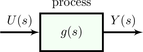
consider the linear, time-invariant system:
with:
- input $U(s)=\mathcal{L}[u(t)]$
- output $Y(s)=\mathcal{L}[y(t)]$
the output for an input is characterized by a transfer function $g(s)=Y(s)/U(s)$.
here, $\mathcal{L}[\cdot]$ is the Laplace transform that maps a function in the time domain $t\in\mathbb{R}$ into the frequency domain $s\in\mathbb{C}$.
a data structure, TransferFunction, represents a transfer function.
constructing a transfer function
for example, consider the transfer function $g(s)=\dfrac{5s+1}{s^2 + 4s+5}$.
constructor 1. we can construct $g(s)$ in an intuitive way that resembles the algebraic expression:
g = (5 * s + 1) / (s ^ 2 + 4 * s + 5) # construction method 1
# output
     5.0*s + 1.0
---------------------
1.0*s^2 + 4.0*s + 5.0
constructor 2. alternatively, we can construct a TransferFunction using the coefficients associated with the powers of $s$ in the polynomials composing the numerator and denominator, respectively, of the rational function $g(s)$. coefficients of the highest powers of $s$ are listed first.
g = TransferFunction([5, 1], [1, 4, 5]) # construction method 2under the hood, s == TransferFunction([1, 0], [1]).
accessing attributes of a transfer function
as rational functions associated with a time delay, each TransferFunction data structure has a numerator, denominator, and time_delay attribute. access as follows:
g.numerator
# output
Polynomial(1.0 + 5.0*s)
g.denominator
# output
Polynomial(5.0 + 4.0*s + 1.0*s^2)g.time_delay
# output
0.0g.numerator and g.denominator are Polynomials from Polynomials.jl.
time delays
to construct a transfer function with a time delay, such as $g(s)=\dfrac{3}{2s+1}e^{-2s}$...
θ = 2.0                              # time delay
g = 3 / (2 * s + 1) * exp(-θ * s)    # construction method 1
g = TransferFunction([3], [2, 1], θ) # construction method 2
# output
    3.0
----------- e^(-2.0*s)
2.0*s + 1.0
zeros, poles, k-factor representation
we can write any transfer function $g(s)$ in terms of its poles ($p_j$), zeros ($z_j$), k-factor ($k$), and time delay ($\theta$):
\[g(s)=k\dfrac{\Pi_j (s-z_j)}{\Pi_j(s-p_j)}e^{-\theta s}\]
the scalar factor $k$ allows us to uniquely specify a transfer function in terms of its poles, zeros, and time delay. note that the $k$-factor is not equal to the zero-frequency gain.
for example, consider:
\[g(s)=\dfrac{5s+1}{s^2 + 4s+5}=5\dfrac{(s+1/5)}{(s+2+i)(s+2-i)}\]
constructing a transfer function from its zeros, poles and k-factor
g = zeros_poles_k([-1/5], [-2 + im, -2 - im], 5.0, time_delay=0.0)  # construction method 3
# output
     5.0*s + 1.0
---------------------
1.0*s^2 + 4.0*s + 5.0
im is the imaginary number $i$. see the Julia docs on complex numbers.
computing the poles, zeros, and k-factor of a transfer function
g = (5 * s + 1) / (s ^ 2 + 4 * s + 5)
z, p, k = zeros_poles_k(g)
# output
([-0.2], ComplexF64[-2.0 - 1.0im, -2.0 + 1.0im], 5.0)
transfer function algebra
add +, subject -, multiply *, and divide / transfer functions.
g₁ = 3 / (s + 2)
g₂ = 1 / (s + 4)
g_product = g₁ * g₂
# output
         3.0
---------------------
1.0*s^2 + 6.0*s + 8.0
g_sum = g₁ + g₂
# output
4.0*s + 14.0
---------------------
1.0*s^2 + 6.0*s + 8.0evaluate a transfer function at a complex number
for example, to evaluate $g(s)=\dfrac{4}{s+2}$ at $s=-2+i$:
g = 4 / (s + 2)
evaluate(g, - 2 + im)
# output
0.0 - 4.0im
zero-frequency gain of a transfer function
compute the zero-frequency gain of a transfer function $g(s)$, which is $g(s)$ evaluated at $s=0$, as follows:
g = (5 * s + 1) / (s ^ 2 + 4 * s + 5)
zero_frequency_gain(g)
# output
0.2
the zero-frequency gain is the ratio of the steady state output value to the steady state input value (e.g., consider a step input). note that the zero-frequency gain could be infinite or zero, which is why we do not have a function to construct a transfer function from its zeros, poles, and zero-frequency gain.
poles, zeros, and zero-frequency gain of a transfer function
compute the poles, zeros, and zero-frequency gain of a transfer function all at once as follows:
g = (5 * s + 5) / (s ^ 2 + 4 * s + 5)
z, p, gain = zeros_poles_gain(g)
# output
([-1.0], ComplexF64[-2.0 - 1.0im, -2.0 + 1.0im], 1.0)
cancel poles and zeros
cancel pairs of identical poles and zeros in a transfer function as follows:
# define g(s) = s * (s+1) / ((s+3) * s * (s+1) ^ 2)
g = TransferFunction([1, 1, 0], [1, 5, 7, 3, 0])
pole_zero_cancellation(g) # 1 / ((s+3) * (s+1))
# output
         1.0
---------------------
1.0*s^2 + 4.0*s + 3.0
under the hood, pole_zero_cancellation compares all pairs of poles and zeros to look for identical pairs via isapprox. after removing identical pole-zero pairs, we reconstruct the transfer function from the remaining poles and zeros–-in addition to its k-factor. we ensure that the coefficients in the resulting rational function are real.
pole-zero cancellation is done automatically when multiplying, dividing, adding, and subtracting transfer functions, as illustrated below.
g = s * (s+1) / ((s+3) * s * (s+1) ^ 2)
# output
         1.0
---------------------
1.0*s^2 + 4.0*s + 3.0
the order of a transfer function
we can find the apparent order of the polynomials in the numerator and denominator of the rational function comprising the transfer function:
g = (s + 1) / ((s + 2) * (s + 3))
system_order(g)
# output
(1, 2)
frequency response of an open-loop transfer function
in the closed loop below, $Y_{sp}$ is the set point for the output, $E$ is the error, and $Y_m$ is the measurement of the output.
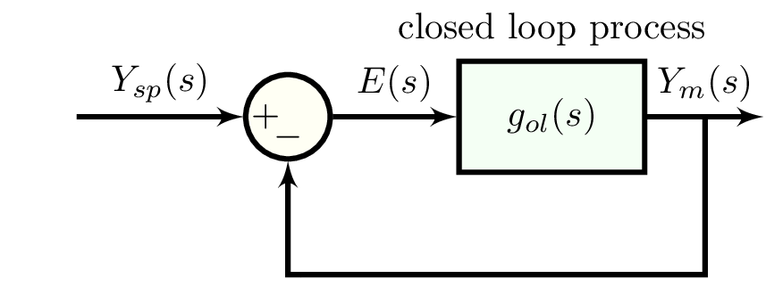
compute the critical frequency, gain crossover frequency, gain margin, and phase margin of a closed loop control system with open-loop transfer function g_ol with gain_phase_margins. for example, consider:
\[g_{ol}(s)=\dfrac{2e^{-s}}{5s+1}\]
g_ol = 2 * exp(-s) / (5 * s + 1)
margins = gain_phase_margins(g_ol)
# output
-- gain/phase margin info--
	critical frequency ω_c [rad/time]:       1.68868
	gain crossover frequency ω_g [rad/time]: 0.34641
	gain margin:                             4.25121
	phase margin:                            1.74798
access the attributes of margins via:
margins.ω_c          # critical freq. (radians / time)
margins.ω_g          # gain crossover freq. (radians / time)
margins.gain_margin  # gain margin
margins.phase_margin # phase margin (radians)
special transfer functions
(0, 1) order transfer functions
\[g(s)=\frac{K}{\tau s +1}\]
easily construct:
K = 2.0
τ = 3.0
g = first_order_system(K, τ)
# output
    2.0
-----------
3.0*s + 1.0
compute time constant:
g = 10 / (6 * s + 2)
time_constant(g)
# output
3.0
(0, 2) order transfer functions
\[g(s)=\frac{K}{\tau^2 s^2 + 2\tau \xi s +1}\]
easily construct:
K = 1.0
τ = 2.0
ξ = 0.1
g = second_order_system(K, τ, ξ)
# output
         1.0
---------------------
4.0*s^2 + 0.4*s + 1.0
compute time constant, damping coefficient:
τ = time_constant(g)
# output
2.0
ξ = damping_coefficient(g)
# output
0.1closed-loop transfer functions
to represent a closed-loop transfer function, we use a special transfer function type, ClosedLoopTransferFunction. this is only necessary when time delays are involved, but it works for when time delays are not involved as well.
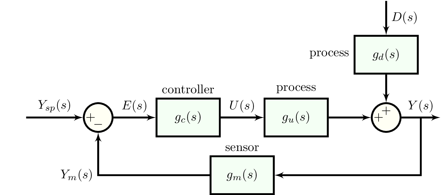
using block diagram algebra, we find the closed-loop transfer functions that relate changes in the output $y$ to changes in the set point $y_{sp}$ and to changes in the disturbance $d$:
\[g_r(s)=\dfrac{Y(s)}{D(s)}=\dfrac{g_d(s)}{1+g_c(s)g_u(s)g_m(s)}\]
\[g_s(s)=\dfrac{Y(s)}{Y_{sp}(s)}=\dfrac{g_c(s)g_u(s)}{1+g_c(s)g_u(s)g_m(s)}\]
we construct these two closed-loop transfer functions as gr and gs as follows.
# PI controller transfer function
pic = PIController(1.0, 2.0)
gc = TransferFunction(pic)

# process, sensor dynamics
gu = 2 / (4 * s + 1) * exp(-0.5 * s)
gm = 1 / (s + 1) * exp(-0.1 * s)
gd = 6 / (6 * s + 1)

# open-loop transfer function
g_ol = gc * gu * gm

# closed-loop transfer function for regulator response
gr = ClosedLoopTransferFunction(gd, g_ol)
# output
closed-loop transfer function.
      top
    -------
    1 + g_ol

  top =
    6.0
-----------
6.0*s + 1.0

  g_ol =
       4.0*s + 2.0
-------------------------- e^(-0.6*s)
8.0*s^3 + 10.0*s^2 + 2.0*s
# closed-loop transfer function for servo response
gs = ClosedLoopTransferFunction(gc * gu, g_ol)
# output
closed-loop transfer function.
top
-------
1 + g_ol
top =
4.0*s + 2.0
--------------- e^(-0.5*s)
8.0*s^2 + 2.0*s
g_ol =
4.0*s + 2.0
-------------------------- e^(-0.6*s)
8.0*s^3 + 10.0*s^2 + 2.0*sdetailed docs
Controlz.TransferFunction — Typetf = TransferFunction([1, 2], [3, 5, 8])
tf = TransferFunction([1, 2], [3, 5, 8], 3.0)construct a transfer function representing a linear, time-invariant system.
example
to construct the transfer function
\[G(s) = \frac{4e^{-2.2s}}{2s+1}\]
in Julia:
tf = TransferFunction([4], [2, 1], 2.2)
# output
    4.0
----------- e^(-2.2*s)
2.0*s + 1.0
attributes
numerator::Polynomial{Float64, :s}: the polynomial in the numerator of the transfer functiondenominator::Polynomial{Float64, :s}: the polynomial in the denominator of the transfer functiontime_delay::Float64: the associated time delay
Controlz.ClosedLoopTransferFunction — Typea closed-loop transfer function that relates an output Y and an input U in a feedback loop.
the resulting closed-loop transfer function is:
 Y      top
--- = --------
 U    1 + g_ol
example
g_ol = 4 / (s + 1) * 2 / (s + 2)
top = 5 / (s + 4)
g = ClosedLoopTransferFunction(top, g_ol)
# output
closed-loop transfer function.
      top
    -------
    1 + g_ol

  top =
    5.0
-----------
1.0*s + 4.0

  g_ol =
         8.0
---------------------
1.0*s^2 + 3.0*s + 2.0
attributes
top::TransferFunction: numeratorg_ol::TransferFunction: open-loop transfer function
Controlz.zero_frequency_gain — FunctionK = zero_frequency_gain(tf)compute the (signed) zero frequency gain of a transfer function $g(s)$, which is:
\[K := \lim_{s\rightarrow 0} G(s)\]
the zero-frequency gain "represents the ratio of the steady state value of the output with respect to a step input" source
example
g = 5 / (3 * s + 1)
K = zero_frequency_gain(g)
# output
5.0
arguments
tf::TransferFunction: the transfer function
returns
K::Float64: the zero-frequency gain of the transfer function
Controlz.zeros_poles_gain — Functionz, p, gain = zeros_poles_gain(tf)Compute the zeros, poles, and zero-frequency gain of a transfer function.
- the zeros are the zeros of the numerator of the transfer function.
- the poles are the zeros of the denominator of the transfer function.
- the zero-frequency gain is the transfer function evaluated at $s=0$
Controlz.zeros_poles_k — Function# compute the zeros, poles, and k-factor of a transfer function
z, p, k = zeros_poles_k(tf)
# construct a transfer function from its zeros, poles, and k-factor
tf = zeros_poles_k(z, p, k, time_delay=0.0)the representation of a transfer function in this context is:
\[g(s)=k\dfrac{\Pi_j (s-z_j)}{\Pi_j (s-p_j)}\]
where $z_j$ is zero $j$, $p_j$ is pole $j$, and $k$ is a constant factor (not equal to the zero-frequency gain) that uniquely specifies the transfer function.
- the zeros are the zeros of the numerator of the transfer function.
- the poles are the zeros of the denominator of the transfer function.
Controlz.pole_zero_cancellation — Functiontf = pole_zero_cancellation(tf, verbose=false, digits=8)find (pole, zero) pairs such that pole = zero and return a new transfer function with those pairs cancelled. this is achieved by comparing the poles and zeros with isapprox, with poles and zeros rounded to digits digits (also applies to reconstruction).
arguments
tf::TransferFunction: the transfer functionverbose::Bool=false: print off which poles, zeros are cancelled.digits::Int: number of digits to round poles and zeros to, for (i) cancelling and (ii) reconstruction.
example
pole_zero_cancellation(s * (s - 1) / (s * (s + 1)))
# output
1.0*s - 1.0
-----------
1.0*s + 1.0Controlz.evaluate — Functionevaluate(tf, z)evaluate a TransferFunction, tf, at a particular number z (could be complex).
example
tf = TransferFunction([1], [3, 1])
evaluate(tf, 1.0)
# output
0.25Controlz.proper — Functionproper(tf)Return true if transfer function tf is proper and false otherwise.
Controlz.strictly_proper — Functionstrictly_proper(tf)Return true if transfer function tf is strictly proper and false otherwise.
Controlz.characteristic_polynomial — Functionp = characteristic_polynomial(g_ol)Determine the characteristic polynomial associated with open loop transfer function g_ol.
The characteristic polynomial is $1+g_{ol}(s)$. The roots of the characteristic polynomial determine the character of the response of the closed loop system to bounded inputs.
Arguments
g_ol::TransferFunction: open loop transfer function
Returns
a polynomial of type Polynomial
Example
g_ol = 4 / (s + 3) / (s + 2) / (s + 1)
characteristic_polynomial(g_ol)
# output
Polynomial(10.0 + 11.0*s + 6.0*s^2 + 1.0*s^3)Controlz.zpk_form — Functiontf = zpk_form(tf)write transfer function tf in zeros, poles, k-factor form:
\[g(s)=k\dfrac{\Pi_j (s-z_j)}{\Pi_j (s-p_j)}\]
where $z_j$ is zero $j$, $p_j$ is pole $j$, and $k$ is a constant factor (not equal to the zero-frequency gain) that uniquely specifies the transfer function.
this is achieved by multiplying by 1.0 in a fancy way such that the highest power of $s$ in the denominator is associated with a coefficient of $1$.
Example
g = 8.0 / (2 * s^2 + 3 * s + 4)
g_zpk = zpk_form(g)
# output
         4.0
---------------------
1.0*s^2 + 1.5*s + 2.0Controlz.system_order — Functiono = system_order(tf::TransferFunction)return the order of the numerator and denominator of the transfer function tf.
use pole_zero_cancellation first if you wish to cancel poles and zeros that are equal before determining the order.
returns
o::Tuple{Int, Int}: (order of numerator, order of denominator)
examples
g = 1 / (s + 1)
system_order(g)
# output
(0, 1)

g = (s + 1) / ((s + 2) * (s + 3))
system_order(g)
# output
(1, 2)Controlz.first_order_system — Functiong = first_order_system(K, τ)construct a first-order transfer function with gain K and time constant τ:
\[g(s)=\frac{K}{\tau s+1}\]
example
K = 1.0
τ = 3.0
g = first_order_system(K, τ)
# output
    1.0
-----------
3.0*s + 1.0
returns
g::TransferFunction: the first order transfer function. well, (0, 1) order.
Controlz.second_order_system — Functiong = second_order_system(K, τ, ξ)construct a second-order transfer function with gain K, time constant τ, and damping coefficient ξ:
\[g(s)=\frac{K}{\tau^2 s^2 + 2\tau \xi s +1}\]
example
K = 1.0
τ = 2.0
ξ = 0.1
g = second_order_system(K, τ, ξ)
# output
         1.0
---------------------
4.0*s^2 + 0.4*s + 1.0
returns
g::TransferFunction: the second order transfer function. well, (0, 2) order.
Controlz.time_constant — Functionτ = time_constant(g)compute the time constant τ of an order (0, 1) or order (0, 2) transfer function.
order (0, 1) representation:
\[g(s)=\frac{K}{\tau s+1}\]
order (0, 2) representation:
\[g(s)=\frac{K}{\tau^2 s^2 + 2\tau \xi s +1}\]
returns
τ::Float64: the time constant.
examples
g = 4 / (6 * s + 2)
time_constant(g)
# output
3.0

g = 1.0 / (8 * s^2 + 0.8 * s + 2)
time_constant(g)
# output
2.0Controlz.damping_coefficient — Functionξ = damping_coefficient(g)compute the damping coefficient ξ of an order (0, 2) transfer function.
order (0, 2) representation:
\[g(s)=\frac{K}{\tau^2 s^2 + 2\tau \xi s +1}\]
returns
ξ::Float64: the damping coefficient
examples
g = 1.0 / (8 * s^2 + 0.8 * s + 2)
damping_coefficient(g)
# output
0.1Controlz.gain_phase_margins — Functionmargins = gain_phase_margins(g_ol, ω_c_guess=0.001, ω_g_guess=0.001)compute critical frequency (radians / time), gain crossover frequency (radians / time), gain margin, and phase margin (radians) of a closed loop, given its closed loop transfer function g_ol::TransferFunction.
if ωc or ωg is not found (i.e. if either are NaN), but the bode_plot clearly shows a critical/gain crossover frequency, adjust ω_c_guess or ω_g_guess to find the root.
Example
g_ol = 2 * exp(-s) / (5 * s + 1)
margins = gain_phase_margins(g_ol)
margins.ω_c # critical freq. (radians / time)
margins.ω_g # gain crossover freq. (radians / time)
margins.gain_margin # gain margin
margins.phase_margin # phase margin (radians)