modeling the shape of a chemical plume
author: Cory Simon, Paul Morris
a mathematical model of a chemical plume
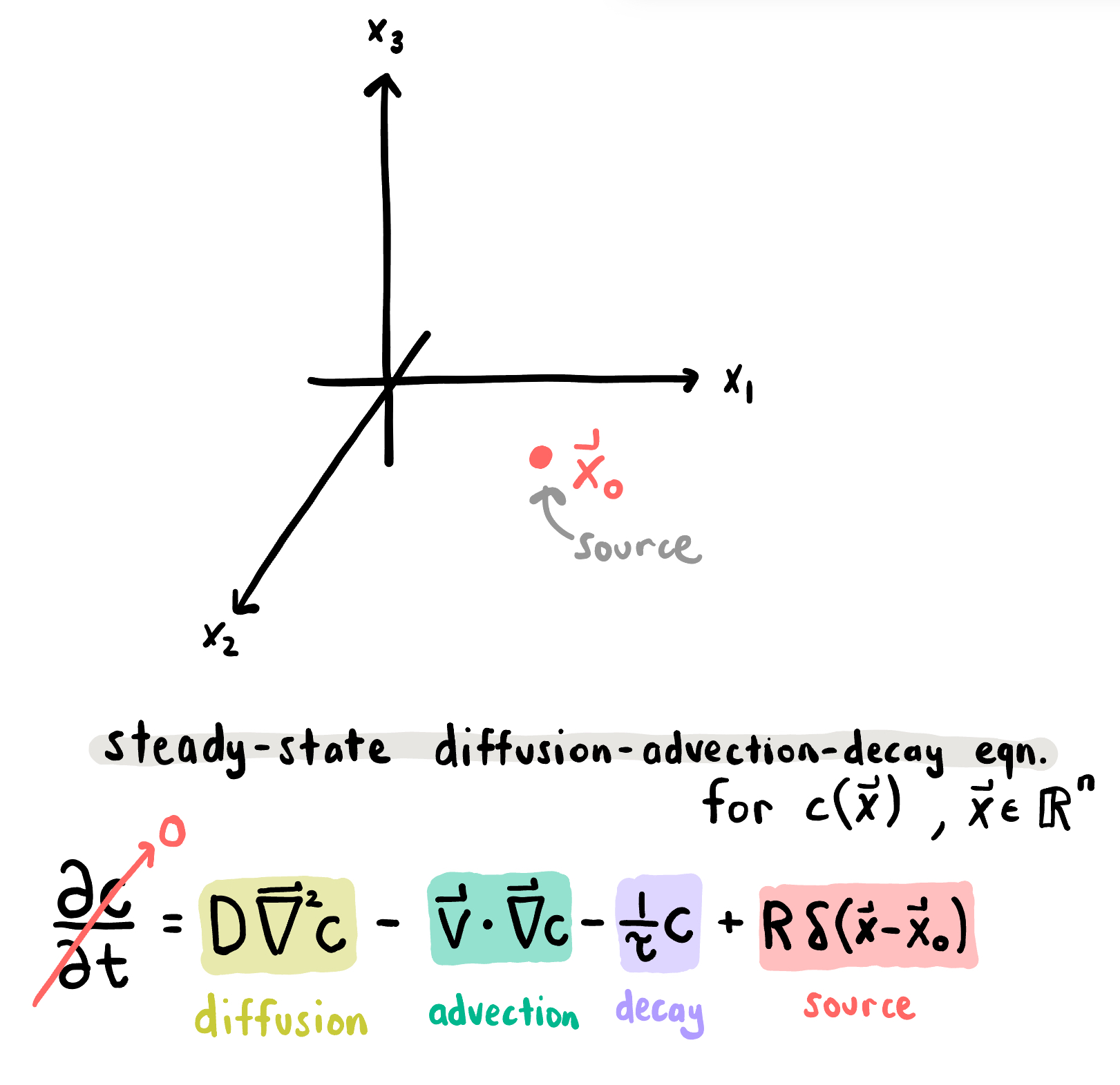
we wish to develop and find the solution to a simple mathematical model of a chemical plume, caused by the continuous release of the chemical from a point source, at steady-state conditions. such a model is useful for (i) predicting the extent and intensity of a chemical plume and (ii) searching for the source of a chemical plume using mobile robots equipped with chemical sensors.
we treat the environment $\mathbb{R}^n$ ($n\in\{2, 3\}$) as spatially homogeneous and aim to account for four pieces of physics:
- the chemical is continuously released into the environment at a constant rate $R$ [g/min] from a point source at location $\mathbf{x}_0\in\mathbb{R}^n$.
- wind transports the chemical downwind through advection, with $\mathbf{v}\in\mathbb{R}^n$ [m/min] the (constant) mean wind vector.
- the chemical diffuses, owing to both molecular diffusivity and [dominant] turbulent diffusivity, with diffusion coefficient $D$ [m$^2$/min].
- the chemical decays, owing to e.g. chemical reaction with humidity or photodegradation, with $\tau$ [min] the mean lifespan of the chemical.
from these simple assumptions, we wish to model the function $c(\mathbf{x})$ [g/m$^n$], the average concentration of the chemical at a point $\mathbf{x}\in\mathbb{R}^n$ in the environment.
the steady-state diffusion-advection-decay equation
applying the law of conservation of mass and accounting for the four pieces of physics listed above, we arrive at the steady-state diffusion-advection-decay [partial differential] equation with a point-source term: $$D {\boldsymbol \nabla}_{\mathbf{x}}^2 c(\mathbf{x}) - \mathbf{v} \cdot {\boldsymbol \nabla}_{\mathbf{x}}c(\mathbf{x}) - \tau^{-1}c(\mathbf{x}) + R \delta(\mathbf{x}-\mathbf{x}_0) = 0$$ respectively, the terms model isotropic diffusivity, advection by wind, decay, and introduction of the chemical into the environment. (here, $\delta(\cdot)$ is the Dirac delta function and e.g. $\boldsymbol \nabla_\mathbf{x}:=[\frac{\partial }{\partial x_1}, \frac{\partial }{\partial x_2}]$ for $n=2$.)
the simple model of the chemical plume at steady state.
(this model is employed in the Infotaxis policy to search for the source of a chemical plume. the equations we derive match those provided in the SI of the Infotaxis paper.)
transformation to the modified Helmholtz equation
we transform the steady-state diffusion-advection-decay equation into a modified Helmholtz problem via the transformation: $$c(\mathbf{x})=:u(\mathbf{x})e^{\mathbf{v}\cdot\mathbf{x} /(2D)}.$$
by the product rule: $${\boldsymbol \nabla}_{\mathbf{x}}c(\mathbf{x})= ({\boldsymbol \nabla}_{\mathbf{x}}u(\mathbf{x}) )e^{\mathbf{v}\cdot\mathbf{x} /(2D)}+ u(\mathbf{x})\mathbf{v}(2D)^{-1}e^{\mathbf{v}\cdot\mathbf{x} /(2D)}.$$ and $${\boldsymbol \nabla}_{\mathbf{x}}^2c(\mathbf{x}) = {\boldsymbol \nabla}_{\mathbf{x}} \cdot {\boldsymbol \nabla}_{\mathbf{x}}c (\mathbf{x})= ({\boldsymbol \nabla}_{\mathbf{x}}^2u(\mathbf{x}) )e^{\mathbf{v}\cdot\mathbf{x} /(2D)}+ ({\boldsymbol \nabla}_{\mathbf{x}} u(\mathbf{x}))\mathbf{v} D^{-1}e^{\mathbf{v}\cdot\mathbf{x} /(2D)} + u(\mathbf{x})(2D)^{-2} \mathbf{v}\cdot \mathbf{v} e^{\mathbf{v}\cdot\mathbf{x} /(2D)}. $$
stuffing these into the original diffusion-advection-decay eqn gives the modified Helmholtz problem in $u(\mathbf{x})$ for $\mathbf{x}\in\mathbb{R}^n$: $${\boldsymbol \nabla}_{\mathbf{x}}^2u - \kappa^2 u = -\frac{R}{D} \delta(\mathbf{x}-\mathbf{x}_0) e^{-\mathbf{v}\cdot\mathbf{x}/(2D)} = -\frac{R}{D} \delta(\mathbf{x}-\mathbf{x}_0) e^{-\mathbf{v}\cdot\mathbf{x_0}/(2D)}$$ with $$\kappa^2:= \frac{\lVert \mathbf{v} \rVert^2+4 \tau^{-1}D}{4D^2}.$$ the latter equality holds because the Dirac delta flattens the exponential term except for at $\mathbf{x}_0$.
note, $\kappa^{-1}$ is a characteristic length-scale governing the dispersion of the chemical.
we now focus on finding the solution $u(\mathbf{x})$ to this modified Helmholtz problem, from which $c(\mathbf{x})$ follows.
solution
the Fourier transform of the modified Helmholtz equation
we take the Fourier transform of the modified Helmholtz problem, giving an algebraic equation in the Fourier transform of $u(\mathbf{x})$, $\tilde{u}(\boldsymbol \omega)$: $$-4 \pi^2\lVert \boldsymbol \omega \rVert^2 \tilde{u}(\boldsymbol \omega) - \kappa^2 \tilde{u}(\boldsymbol \omega)= -\frac{R}{D}e^{-2\pi i \boldsymbol\omega \cdot \mathbf{x}_0}e^{-\mathbf{v}\cdot\mathbf{x_0}/(2D)}$$ we solve for the solution in the frequency domain: $$\tilde{u}(\boldsymbol \omega) = \dfrac{\frac{R}{D}e^{-\mathbf{v}\cdot\mathbf{x}_0 / (2D)}}{4\pi^2 \lVert \boldsymbol \omega \rVert^2 + \kappa^2}e^{-2\pi i \boldsymbol\omega \cdot \mathbf{x}_0}.$$
the inverse Fourier transform
to obtain $u(\mathbf{x})$, we take the inverse Fourier transform of $\tilde{u}(\boldsymbol \omega)$: $$u(\mathbf{x}) = \int_{\mathbb{R}^n} \dfrac{\frac{R}{D}e^{-\mathbf{v}\cdot\mathbf{x}_0 / (2D)}}{4\pi^2 \lvert \boldsymbol \omega \rvert^2 + \kappa^2}e^{-2\pi i \boldsymbol\omega \cdot \mathbf{x}_0}e^{2\pi i \boldsymbol \omega \cdot \mathbf{x}} d\boldsymbol\omega.$$
the $e^{-2\pi i \boldsymbol\omega \cdot \mathbf{x}_0}$ term corresponds to a translation, so let’s focus on:
$$u(\mathbf{x}+\mathbf{x}_0) = \frac{R}{D}e^{-\mathbf{v}\cdot\mathbf{x}_0 / (2D)} \int_{\mathbb{R}^n} \dfrac{ e^{2\pi i \boldsymbol \omega \cdot \mathbf{x}} }{4\pi^2 \lVert \boldsymbol \omega \rVert^2 + \kappa^2}d\boldsymbol\omega.$$
now, the approach to evaluate the integral $$I_n(\mathbf{x}):= \int_{\mathbb{R}^n} \dfrac{ e^{2\pi i \boldsymbol \omega \cdot \mathbf{x}} }{4\pi^2 \lVert \boldsymbol \omega \rVert^2 + \kappa^2}d\boldsymbol\omega$$ is qualitatively different depending on the dimension of the space, $n$. so, we treat $n=2$ and $n=3$ separately below.
case $n=3$
we write the integral $I_3(\mathbf{x})$ in spherical coordinates $(\rho, \phi, \theta)$ with $\rho=\lVert \boldsymbol\omega\rVert$ the radius, $\phi$ the polar angle, and $\theta$ the azimuthal angle. aligning the $z$-axis of this spherical coordinate system with the vector $\mathbf{x}$, we can write: $$\mathbf{x}\cdot \boldsymbol \omega= \lVert \mathbf{x} \lVert \lVert \boldsymbol \omega \lVert \cos \phi$$ and the integral becomes (the volume element in spherical coordinates is $\rho^2\sin \phi d\rho d\phi d\theta$):
$$ I_3(\mathbf{x})= \int_0^{2\pi} \int_0^{\pi} \int_0^{\infty} \dfrac{ e^{2\pi i \rho \lVert \mathbf{x}\rVert \cos \phi } }{4\pi^2 \rho^2 + \kappa^2} \rho^2 \sin \phi d\rho d\phi d\theta $$
right away, we can knock out the integral in $\theta$ as $2\pi$ and tackle the integral in $\phi$ with a simple substitution $\xi := \cos \phi$ giving: $$ I_3(\mathbf{x})= \int_0^{\infty} \frac{1}{i \lVert \mathbf{x} \rVert} \left(e^{2\pi i \rho \lVert \mathbf{x}\rVert } - e^{-2\pi i \rho \lVert \mathbf{x}\rVert }\right) \dfrac{\rho }{4\pi^2 \rho^2 + \kappa^2} d\rho $$
breaking the integral into a sum of two integrals $$ I_3(\mathbf{x})= \frac{1}{i \lVert \mathbf{x} \rVert}\left( \int_0^{\infty} e^{2\pi i \rho \lVert \mathbf{x}\rVert } \dfrac{\rho }{4\pi^2 \rho^2 + \kappa^2} d\rho- \int_0^{\infty} e^{-2\pi i \rho \lVert \mathbf{x}\rVert } \dfrac{\rho }{4\pi^2 \rho^2 + \kappa^2} d\rho \right) $$
and doing a $\hat{\rho}:=-\rho$ substitution in the second integral allows us to write this as a single integral: $$ I_3(\mathbf{x})= \frac{1}{i \lVert \mathbf{x} \rVert} \int_{-\infty}^{\infty} e^{2\pi i \rho \lVert \mathbf{x}\rVert } \dfrac{\rho }{4\pi^2 \rho^2 + \kappa^2} d\rho. $$
we tackle this integral by involving it in a contour integration in the complex plane $\mathbb{C}$. consider the simple, directed, closed curve $\gamma$ in $\mathbb{C}$ consisting of (1) a line segment on the real axis from $-R$ to $R$ followed by (2) the upper semicircle of radius $R$, centered at $0$. we choose $R> \kappa/(2\pi)$ so the contour $\gamma$ encloses the pole (one of two) $z=\kappa/(2\pi)i$ of the integrand (now viewed as a complex function) $$g(z):=e^{2\pi i z \lVert \mathbf{x}\rVert } \dfrac{z }{4\pi^2 z^2 + \kappa^2}, z \in \mathbb{C}.$$
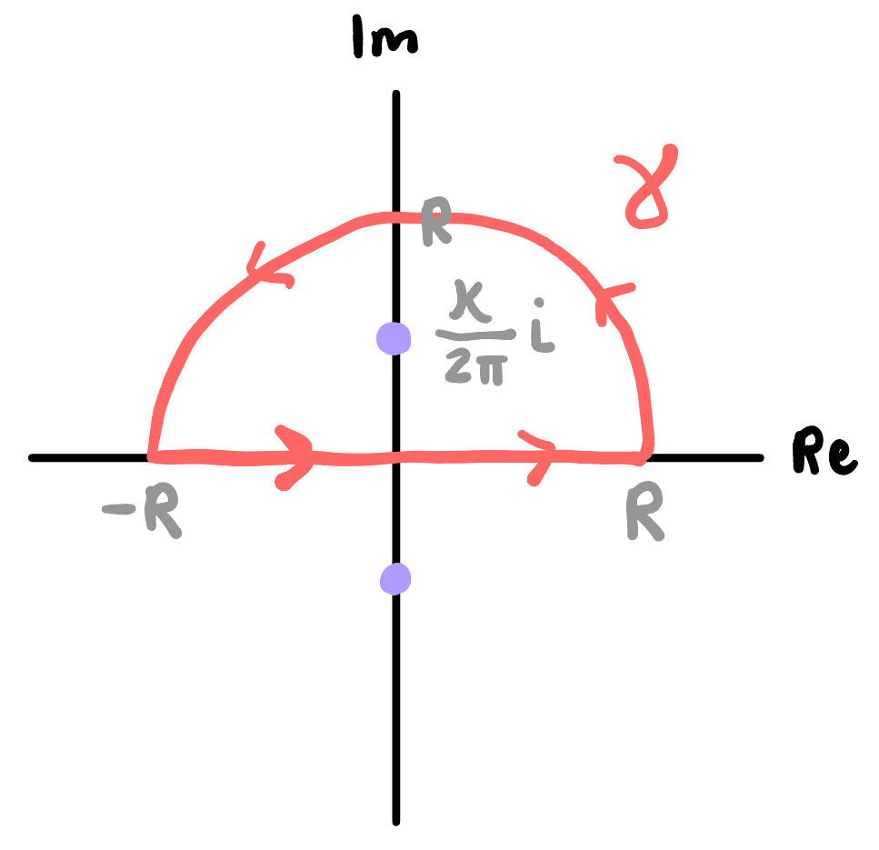
the contour $\gamma$ together with the two poles of $g(z)$.
we can break the contour integral into two pieces: $$ \frac{1}{i \lVert \mathbf{x} \rVert} \oint_{\gamma}g(z)dz = \frac{1}{i \lVert \mathbf{x} \rVert} \int_{-R}^R g(z) dz + \frac{1}{i \lVert \mathbf{x} \rVert} \int_{\{Re^{i\theta} :\, 0 \leq \theta \leq \pi\}} g(z)dz $$
now, as $R\rightarrow\infty$, the second integral becomes $I_3(\mathbf{x})$ we’re looking for. and, via Jordan’s lemma, $\int_{\{Re^{i\theta} :\, 0 \leq \theta \leq \pi\}}g(z) dz \rightarrow 0$ as $R\rightarrow \infty$. so: $$ \frac{1}{i \lVert \mathbf{x} \rVert} \lim_{R\rightarrow\infty} \oint_{\gamma(R)}g(z)dz = I_3(\mathbf{x}), $$ where we note the contour $\gamma$ depends on $R$.
via Cauchy’s residue theorem: $$\oint_{\gamma}g(z)dz=2\pi i \text{Res}(g, \kappa/(2\pi)i)$$ since the contour $\gamma$ encircles the pole $\kappa/(2\pi)i$ of the complex function $g(z)$ in a counter-clockwise fashion.
calculating the residue: $$\text{Res}(g, \kappa/(2\pi)i)=\lim_{z\rightarrow \kappa/(2\pi)i}(z-\kappa/(2\pi)i)g(z)=\frac{1}{8\pi^2}e^{-\kappa \lVert \mathbf{x} \rVert}$$
finally, then: $$ I_3(\mathbf{x})= \int_{\mathbb{R}^2} \dfrac{ e^{2\pi i \boldsymbol \omega \cdot \mathbf{x}} }{4\pi^2 \lvert \boldsymbol \omega \rvert^2 + \kappa^2}d\boldsymbol\omega = \frac{1}{4\pi \lVert \mathbf{x} \rVert}e^{-\kappa\lVert \mathbf{x}\rVert}. $$
and we have: $$u(\mathbf{x})=\frac{R}{4\pi D} \frac{1}{\lVert \mathbf{x}-\mathbf{x}_0\rVert} e^{-\kappa \lVert \mathbf{x}-\mathbf{x}_0\rVert}e^{-\mathbf{v} \mathbf{x}_0/(2D)}$$
going back to $c(\mathbf{x})$, finally, we have the shape of the chemical plume in 3D!
$$\boxed{c(\mathbf{x})=\frac{R}{4\pi D} \frac{1}{\lVert \mathbf{x}-\mathbf{x}_0\rVert} e^{-\kappa \lVert \mathbf{x}-\mathbf{x}_0\rVert}e^{\mathbf{v} \cdot (\mathbf{x}-\mathbf{x}_0)/(2D)}, \mathbf{x}\in\mathbb{R}^3.}$$
case $n=2$
we write the integral $I_2(\mathbf{x})$ in polar coordinates $(r, \theta)$ with $r=\lVert \boldsymbol\omega\rVert$ the radius and $\theta$ the angle. aligning the $x$-axis of this polar coordinate system with the vector $\mathbf{x}$, we can write: $$\mathbf{x}\cdot \boldsymbol \omega= \lVert \mathbf{x} \lVert \lVert \boldsymbol \omega \lVert \cos \theta$$ and the integral becomes (the area element in polar coordinates is $r drd\theta$): $$ I_2(\mathbf{x})= \int_0^{2\pi} \int_0^{\infty} \dfrac{ e^{2\pi i r \lVert \mathbf{x}\rVert \cos \theta } }{4\pi^2 r^2 + \kappa^2} r dr d\theta $$
we recognize the integral over $\theta$ as a function of $\lVert \mathbf{x} \rVert$ as related to the zero-order Bessel function of the first kind, whose integral representation (Hansen-Bessel formula) is: $$J_0(a):=\frac{1}{\pi} \int_0^\pi e^{i a \cos(\theta)}d\theta.$$ by the power series representation of $J_0(a)$, it is an even function i.e. $J_0(a)=J_0(-a)$. so: $$\int_0^{2\pi} e^{i a \cos(\theta)}d\theta= \int_0^{\pi} e^{i a \cos(\theta)}d\theta+\int_\pi^{2\pi} e^{i a \cos(\theta)}d\theta=\pi J_0(a) + \int_0^{\pi} e^{-i a \cos(\theta)}d\theta = 2\pi J_0(a)$$
so, we can involve $J_0(\cdot)$ in $I_2(\mathbf{x})$: $$ I_2(\mathbf{x})= \int_0^{\infty} \dfrac{ r }{4\pi^2 r^2 + \kappa^2} 2\pi J_0(2\pi r \lVert \mathbf{x}\rVert) r dr= \frac{1}{2\pi} \int_0^{\infty} \dfrac{ r }{r^2 + (\kappa/2\pi)^2} J_0(2\pi r \lVert \mathbf{x}\rVert) r dr $$
next, we recognize this as resembling the Hankel-Nicholson integral (eqn 11.4.44 in Abramowitz and Stegun): $$\int_0^\infty \frac{r}{r^2+\xi ^2}J_0(ar) dr=K_0(a\xi)$$ where $K_0(\cdot)$ is the zero-order modified Bessel function of the second kind (we suspect, the proof of this follows from the series representations of $J_0(\cdot)$ and $K_0(\cdot)$). this gives: $$ I_2(\mathbf{x})= \frac{1}{2\pi} K_0(\kappa \lVert \mathbf{x} \rVert). $$
(many numerical libraries, e.g. Python and Julia, provide implementations of $K_0(\cdot)$. e.g. Scipy.)
finally, using $I_2(\mathbf{x})$ to construct $u(\mathbf{x})$, then using $u(\mathbf{x})$ to construct $c(\mathbf{x})$, we have the shape of the chemical plume in 2D! $$\boxed{ c(\mathbf{x})= \frac{R}{2\pi D} K_0(\kappa \lVert \mathbf{x}-\mathbf{x}_0\rVert)e^{\mathbf{v} \cdot (\mathbf{x}-\mathbf{x}_0)/(2D)} , \mathbf{x} \in \mathbb{R}^2}$$
visualization
we use Julia to visualize the shape of the chemical plume in 2D.
first, we define a data structure to store the parameters characterizing the chemical plume.
struct PlumeParams
    x₀::Vector{Float64} # source location [m]
    R::Float64          # source strength [g/min]
    v::Vector{Float64}  # wind vector [m/s]
    D::Float64          # diffusion coefficent [m²/min]
    τ::Float64          # lifespan [min]
    κ::Float64          # m⁻²
end

# constructor that computes κ for us
function PlumeParams(; x₀=x₀, R=R, D=D, τ=τ, v=v)
    κ = sqrt((dot(v, v) + 4 * D / τ) / (4 * D ^ 2)) # m⁻²
    return PlumeParams(x₀, R, v, D, τ, κ)
end
second, we use the SpecialFunctions.jl implementation of the zero-order modified Bessel function of the second kind to define the function $c(\mathbf{x})$ for $\mathbf{x}\in\mathbb{R^2}$.
function c(x::Vector{Float64}, p::PlumeParams) # g/m²
	return p.R / (2 * π * p.D) * besselk(0, p.κ * norm(x - p.x₀)) *
	        exp(dot(p.v, x - p.x₀) / (2 * p.D))
end
third, we compute $c(\mathbf{x})$ over a grid of points in $\mathbb{R}^2$.
L = 50.0 # m
res = 500
xs = range(0.0, L, length=res) # m
p = PlumeParams(x₀=[25.0, 4.0], R=10.0, D=25.0, τ=50.0, v=[-5.0, 15.0])

cs = [c([x₁, x₂], p) for x₁ in xs, x₂ in xs] # g/m²
finally, we visualize the plume with CairoMakie.jl:
cmap = ColorScheme(
    vcat(
        ColorSchemes.grays[end],
        reverse([ColorSchemes.viridis[i] for i in 0.0:0.05:1.0])
    )
)

fig = Figure()
ax  = Axis(
    fig[1, 1],
    aspect=DataAspect(),
    xlabel="x₁",
    ylabel="x₂"
)
hm  = heatmap!(xs, xs, cs, colormap=cmap, colorrange=(0.0, maximum(cs)))
Colorbar(fig[1, 2], hm, label = "concentration c(x₁, x₂) [g/m²]")
fig
voila!
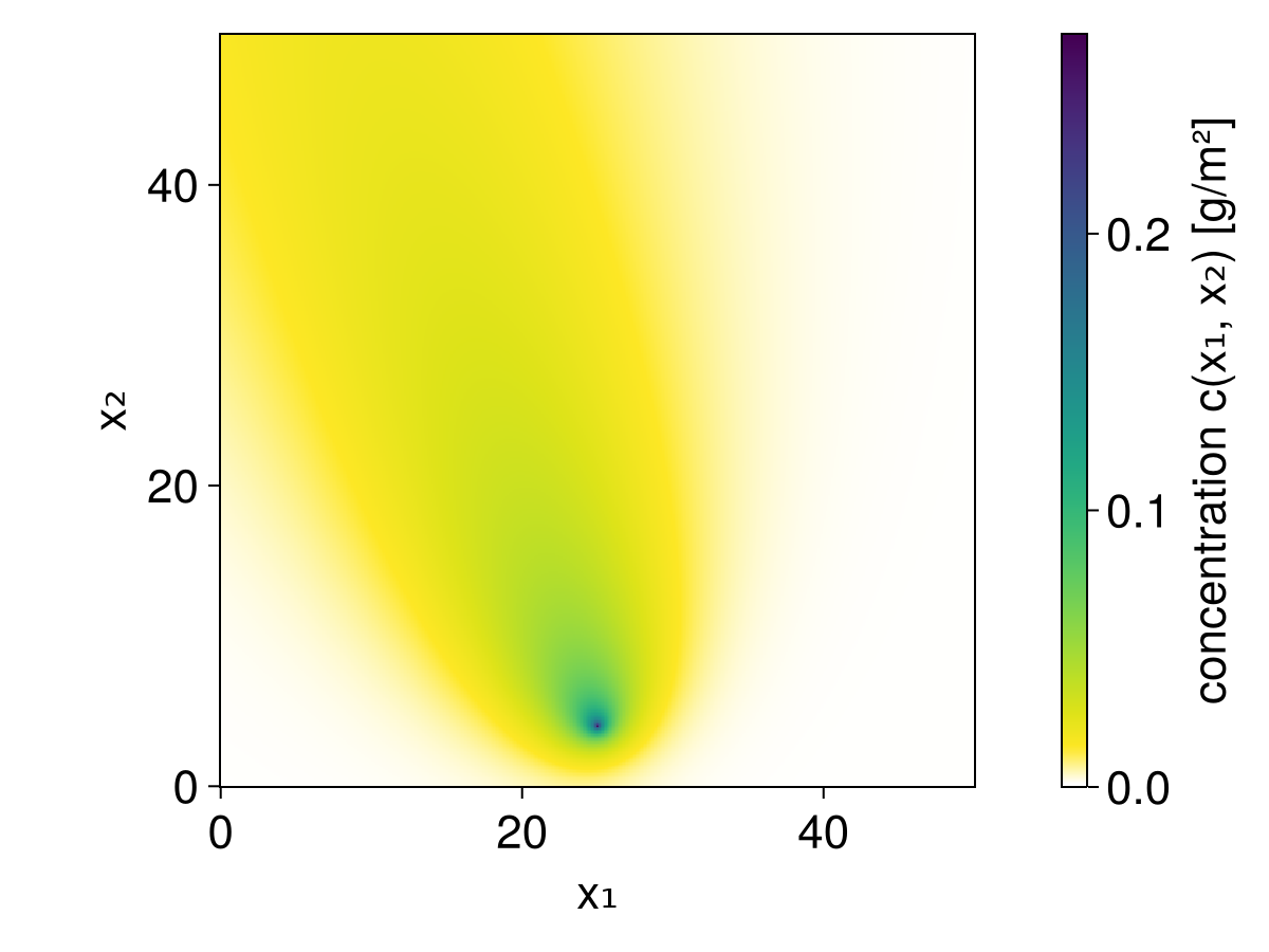
visualization of $c(\mathbf{x})$ for $\mathbf{x}\in\mathbb{R}^2$.
modeling the sensor
we now model how a chemical sensor, on a mobile robot at position $\mathbf{x}$, detects the chemical. we’ve established the mean concentration $c(\mathbf{x})$ in the environment, but at the smaller scale near the sensing element, there will be a concentration gradient owing to adsorption/reaction of the gas on the surface of the sensing element.
we consider the $n=2$ case only.
we assume:
- the surface of the sensing element:
- is a circle of radius $a$.
- presents binding sites that adsorb and catalyze degradation of the chemical from the gas phase. so, the concentration of gas near the sensing element is zero.
- sufficiently far from the surface of the sensor, the concentration in the gas is that in the bulk, $c(\mathbf{x})$.
- steady-state conditions.
treating only the diffusion at this length-scale, the concentration near the sensor is radially symmetric, with $c_s(r)$ with $r \in [0, \kappa^{-1}]$ the distance from the sensor, satisfies the steady-state diffusion equation in polar coordinates: $$\frac{\mathrm{d}^2c_s}{\mathrm{d}r^2}+\frac{1}{r}\frac{\mathrm{d}c_s}{\mathrm{d}r} =\frac{1}{r}\frac{\mathrm{d}}{\mathrm{d}r} \left( r\frac{\mathrm{d} c_s}{\mathrm{d} r}\right) = 0$$ integrating twice then applying the boundary conditions $c_s(a)=0$ and $c_s(\kappa^{-1})=c(\mathbf{x})$, with the length-scale $\kappa^{-1}$ dictating how far from the sensor the concentration equals the bulk, gives: $$c_s(r) = c(\mathbf{x}) \frac{\log(r/a)}{\log(\kappa^{-1}/a)}.$$
now, the response/signal from the chemical sensor is proportional to the flux of gas impinging on its surface, due to diffusion. multiplying by the circumference of the sensor gives the rate at which gas molecules impinge onto the sensing element: $$J=(2\pi a)D\frac{\mathrm{d} c_s}{\mathrm{d} r} \bigg \rvert_{r=a}.$$ this gives us eqn. (7) in the SI of the Infotaxis paper: $$J(\mathbf{x})=\frac{R}{\log(\kappa^{-1}/a)}K_0(\kappa \lVert \mathbf{x}-\mathbf{x}_0\rVert)e^{\mathbf{v} \cdot (\mathbf{x}-\mathbf{x}_0)/(2D)}.$$
thus, when a sensor stays at position $\mathbf{x}$ for a duration $\Delta t$ to detect the chemical, we expect $J(\mathbf{x})\Delta t$ g of the chemical to be detected.
appendix
the Fourier transform
definition
the Fourier transform of a function $f(\mathbf{x})$ is defined as: $$\mathcal{F}[f(\mathbf{x})] ({\boldsymbol \omega}):=\int_{\mathbb{R}^n} f(\mathbf{x}) e^{-2\pi i {\boldsymbol \omega}}d\mathbf{x} =: \tilde{f}({\boldsymbol \omega})$$ where ${\boldsymbol \omega}\in\mathbb{R}^n$.
inverse Fourier transform
for recovering the function $f(\mathbf{x})$ from its Fourier transform $\tilde{f}(\boldsymbol \omega)$, the inverse Fourier transform is: $$f(\mathbf{x})=\mathcal{F}^{-1}[f({\boldsymbol \omega})] (\mathbf{x}) :=\int_{\mathbb{R}^n} \tilde{f}({\boldsymbol \omega}) e^{2\pi i {\boldsymbol \omega}}d\mathbf{x}.$$
Fourier transform of a Dirac delta function
via the sifting property of the Dirac delta function $$\mathcal{F}[\delta(\mathbf{x}-\mathbf{x}_0)] ({\boldsymbol \omega}) := \int_{\mathbb{R}^n} \delta (\mathbf{x} - \mathbf{x}_0) e^{-2\pi i {\boldsymbol \omega}}d\mathbf{x} = e^{-2\pi i \mathbf{x}_0}.$$
Fourier transform of derivatives
the Fourier transform of a derivative is: $$\mathcal{F}\left[\frac{\partial f}{\partial x_i}\right] ({\boldsymbol \omega}) := \int_{\mathbb{R}^n} \frac{\partial f}{\partial x_i} e^{-2\pi i {\boldsymbol \omega}}d\mathbf{x}.$$ tackling the integral over $x_i \in (-\infty, \infty)$ by parts, with $u:=e^{-2\pi i \boldsymbol \omega}$ and $dv=\frac{\partial f}{\partial x_i} dx_i$ gives, provided $f \rightarrow 0$ as $x_i \rightarrow \pm \infty$: $$\mathcal{F}\left[\frac{\partial f}{\partial x_i}\right] ({\boldsymbol \omega}) = 2 \pi i \omega_i \tilde{f}(\boldsymbol \omega).$$ hence, $$\mathcal{F}\left[{\boldsymbol \nabla}_{\mathbf{x}} f \right] ({\boldsymbol \omega}) = 2 \pi i {\boldsymbol \omega} \tilde{f}(\boldsymbol \omega)$$ and $$\mathcal{F}\left[{\boldsymbol \nabla}_\mathbf{x}^2 f \right] ({\boldsymbol \omega}) = -4 \pi^2 {\boldsymbol \omega} \cdot {\boldsymbol \omega} \tilde{f}(\boldsymbol \omega) = -4\pi^2 \lVert \boldsymbol \omega \rVert^2 \tilde{f}(\boldsymbol \omega).$$
Fourier transform of a translated function
finally, we remark that a translation of the function $f(\mathbf{x})$ by vector $\mathbf{x}_0$ gives: $$\mathcal{F}[f(\mathbf{x}-\mathbf{x}_0)] ({\boldsymbol \omega}) := \int_{\mathbb{R}^n} f (\mathbf{x} - \mathbf{x}_0) e^{-2\pi i {\boldsymbol \omega}}d\mathbf{x} = e^{-2\pi i \mathbf{x}_0} \tilde{f}(\boldsymbol \omega).$$ shown after a substitution $\mathbf{x}^\prime:=\mathbf{x}-\mathbf{x}_0$. hence, $$\mathcal{F}^{-1}[f({\boldsymbol \omega})e^{-2\pi i \mathbf{x}_0}] (\mathbf{x}) = f(\mathbf{x}-\mathbf{x}_0).$$
references
- “n-dimensional Fourier Transform, Ch. 8” notes by Prof. Brad Osgood. link
- Vergassola, M., Villermaux, E., & Shraiman, B. I. (2007). ‘Infotaxis’ as a strategy for searching without gradients. Nature, 445 (7126), 406-409.
- Loisy, Aurore, and Christophe Eloy. “Searching for a source without gradients: how good is infotaxis and how to beat it.” Proceedings of the Royal Society A 478, no. 2262 (2022): 20220118.
- Yukawa Potential hw assignment from Dept. of Physics at Montana State University. here
- Digital Library of Mathematical Functions, Ch. 10: Bessel Functions. link
- Abramowitz and Stegun. (1965). Handbook of Mathematical Functions.