the German tank problem
author: Cory Simon
The German tank problem [1] is intellectually stimulating and makes great conversation at wine bars. The problem has a historical context as well [2].
During World War 2, the Germans inscribed their tanks with sequential serial numbers $1,2,…,n$ when they were manufactured. The total number of tanks $n$ that the Germans had, however, was unknown to the Allied forces– and of great interest.
The Allies captured a (assumed) random sample of $k$ tanks from the German forces (without replacement, of course) and observed their serial numbers, $x_1,x_2,…,x_k$. The German tank problem is to estimate the total number of tanks $n$ from the observed serial numbers $x_1,x_2,…,x_k$.
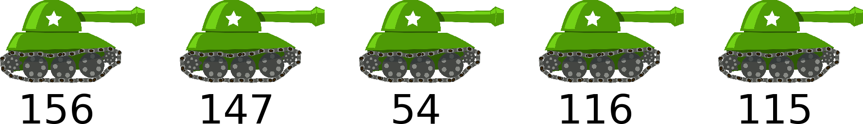
A random sample (without replacement) of German tanks and their inscribed serial numbers. Based on this outcome, how many tanks do you estimate the Germans have?
The number of tanks is of course greater than or equal to the maximum serial number observed ($n \geq \max x_i$); given the sample above, estimating that the Germans have fewer than 156 tanks would be absurd. However, estimating that the Germans have 156 tanks seems too conservative; this estimate assumes that we happened to capture the most recently manufactured tank. Intuitively, we should estimate the total number of tanks to be 156 plus some number to reflect the small likelihood that we captured the very last tank to come out of the factory (as opposed to not capturing it). How large should this number be?
Let’s now delve into the math to answer this question, but feel free to skip to # an unbiased estimator.
the data generating process (dgp)
Think of tank capturing as a stochastic process governed by an underlying data generating process (dgp). The data are the set of serial numbers $\{x_1,x_2,…,x_k\}$. The dgp is a uniform random selection, without replacement, from the set of integers $\{1,2,…,n\}$. This is our model for the stochastic process of capturing tanks.
Because all viable outcomes (sets of observed serial numbers) are equally probable, the probability of any particular viable outcome, given we know $n$, is: $$P({x_1, x_2, …, x_k} | n)=\dfrac{1}{\binom{n}{k}}$$ A viable outcome is one where $x_i \in {1, 2, …, n}$ for all $i\in {1,2,…,k}$. So our dgp is governed by the probability distribution above, which is a uniform distribution over the sample space. The denominator is the cardinality of the sample space– how many ways we can select $k$ integers from $n$ without replacement, given the order in which they were selected does not matter.
simulating the German tank problem in Julia
Let’s simulate the dgp in the Julia programming language. For elegance, let’s first define a data structure for a tank.
struct Tank
    serial_nb::Int
end

tank = Tank(4) # construct tank with serial number 4.
The following function uses the sample function in StatsBase.jl to simulate tank capture. It returns an array of Tanks that were captured.
function capture_tanks(nb_tanks_captured::Int, nb_tanks::Int)
    #  construct array of tanks w serial numbers 1,2,...,nb_tanks
    tanks = [Tank(serial_nb) for serial_nb = 1:nb_tanks]
    # return a random selection of these tanks w./o replacement
    return sample(tanks, nb_tanks_captured, replace=false)
end

captured_tanks = capture_tanks(5, 300) # an array of captured tanks
We’ll use this function to simulate tank capture and assess two different estimators for the number of tanks.
what is an estimator?
An estimator maps an outcome of a random experiment to an estimate of a parameter that characterizes the underlying dgp. In the German tank problem, the outcome is a set of serial numbers on the captured tanks, $\{x_1, x_2, …, x_k\}$, and the parameter in the dgp we estimate, from the outcome, is the total number of tanks, $n$. We already discussed one estimator of $n$ for the German tank problem: the maximum observed serial number $m\equiv \max x_i$.
We aim to derive an unbiased estimator, meaning that, on average, the estimator recovers the true value of the parameter in the dgp. The average here is over the ensemble of possible outcomes generated by the dgp.
The maximum serial number $m$ is a biased estimator because it is either equal to the true value of $n$ (if we happen to capture the most recently manufactured tank) or an underestimate. To illustrate this, I ran 100,000 simulations of our dgp using the capture_tanks function with $n=100$ and $k=5$. The histogram below shows the distribution of the estimated number of tanks using the estimator $m \equiv \max x_i$.
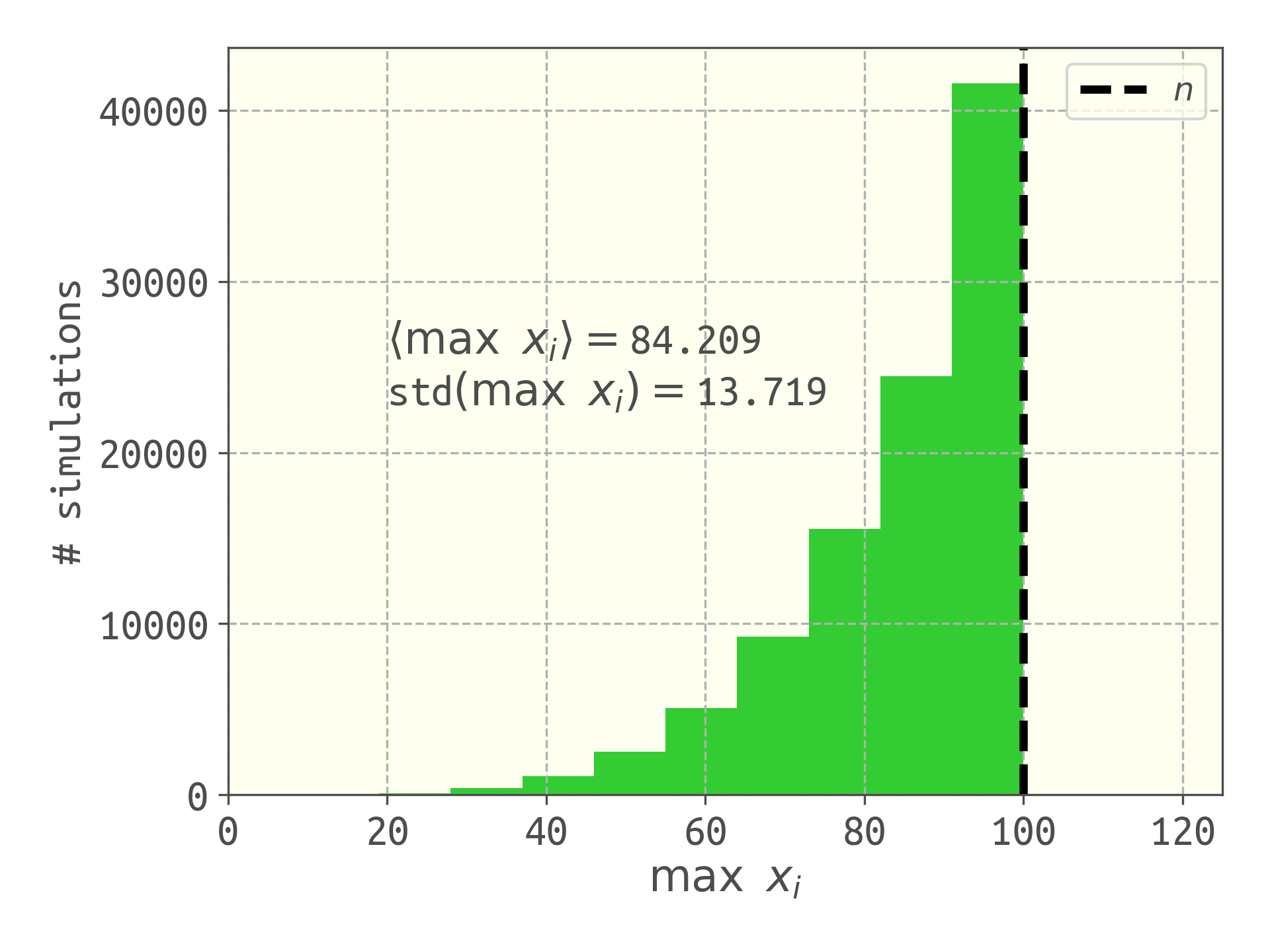
The maximum serial number observed is a biased estimator of $n$; the average of the estimate over 10,000 simulations is less than the true number of tanks, $n$.
pursuing an unbiased estimator of $n$
Let us proceed to derive an unbiased estimator based on the maximum serial number observed, $m$. We will find out what number to add to $m$ to arrive at an unbiased estimate of $n$.
the likelihood $Pr(M=m|n)$
Let $M$ be the random variable that is the maximum serial number. We wish to derive the probability that the max serial number is $m$, given the total number of tanks is $n$, $Pr(M=m|n)$. Because the dgp is a uniform probability on the sample space, $$Pr(M=m|n)=\dfrac{|\text{subset of sample space such that } m=\max x_i|}{|\text{sample space}|}$$
The cardinality of the sample space, we argued, is $\binom{n}{k}$. The schematic below illustrates that the cardinality of the subset of the sample space such that the max serial number is $m$ is $\binom{m-1}{k-1}$. i.e., if the max serial number is $m$, this gives us $k-1$ remaining tanks to select from the $m-1$ tanks with a serial number less than $m$. $$Pr(M=m|n) = \dfrac{\binom{m-1}{k-1}}{\binom{n}{k}}$$ This distribution pertains only to $m$ such that $n \geq m\geq k$ since the max serial number cannot be more than the total number of tanks or less than the number of captured tanks.
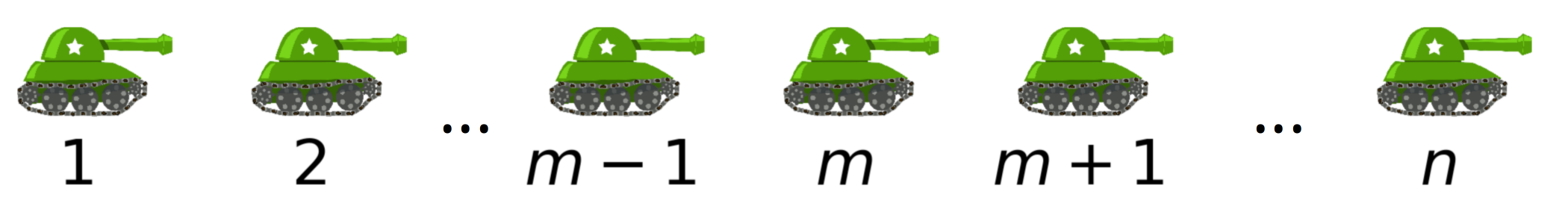
Count the number of sets of $k$ serial numbers such that the maximum serial number is $m$. Obviously, one of the $k$ captured tanks must have serial number $m$. Then, the remaining $k-1$ tanks must have been selected from the $m-1$ tanks preceding the tank with the max serial number $m$. Thus, the number of outcomes such that the max serial number is $m$ is equal to the number of ways to choose $k-1$ tanks from $m-1$ labeled tanks, without replacement, where order does not matter.
a useful identity from the normalization of the probability mass function
Since $n \geq m \geq k$: $$1= \sum_{m=k}^n Pr(M=m|n) = \sum_{m=k}^n \dfrac{\binom{m-1}{k-1}}{\binom{n}{k}}$$ i.e. the probability that $m$ is (inclusive) between $k$ and $m$ is one. The $P(M=m|n)$ sum to one because the event that the max serial number is $\theta$ is independent from the event that the max serial number is $\beta \neq \theta$. This gives us an identity that we will use later: $$\binom{n}{k} = \sum_{m=k}^n \binom{m-1}{k-1}$$
This identity has an intuitive interpretation. The sample space for the German tank problem is the union of the following disjoint sets of outcomes: the set of outcomes where the max serial number $m$ is $k$, the set of outcomes where the max serial number is $k+1$, …, the set of outcomes where the max serial number is $n$.
the expected value of the max serial number, $E(M=m|n)$
Now let us find the expected value of $M$ over the outcomes of our dgp. $$E(M | n) = \displaystyle \sum_{m=k}^n m Pr(M=m|n)$$ We’re conditioning on knowing $n$, which seems awkward because the whole point of the German tank problem is that we don’t know $n$. Our strategy here is to find $E(M | n)$, then find what $n$ gives an expected value of $M$ equal to the $m$ we observed. This gives an unbiased estimator for $n$. Using our expression for $Pr(M=m|n)$ above: $$E(M | n) = \sum_{m=k}^n m \frac{\binom{m-1}{k-1}}{\binom{n}{k}}$$ The sum is over $m$, so we can pull the denominator outside of the sum. Also, we can write this as a sum over combinations by multiplying by one in a fancy way and absorbing the $m$ and $k$ into the factorial terms: $$E(M | n) = \dfrac{1}{\binom{n}{k}} \sum_{m=k}^n \frac{k}{k} m \frac{(m-1)!}{(k-1)!(m-k)!}$$ $$E(M | n) = \dfrac{k}{\binom{n}{k}} \sum_{m=k}^n \frac{m!}{k!(m-k)!}$$ $$E(M | n) = \dfrac{k}{\binom{n}{k}} \sum_{m=k}^n \binom{m}{k}$$
The sum can be simplified by writing our identity above for a situation where we select $k+1$ tanks from a population of $n+1$ tanks: $$\binom{n+1}{k+1} = \sum_{m=k+1}^{n+1} \binom{m-1}{k}$$ since then the max serial number can run from $k+1$ to $n+1$, and the remaining $k$ tanks must have serial numbers less then $m$. A change of variables $\theta := m -1$ then gives: $$\binom{n+1}{k+1} = \sum_{\theta=k}^{n} \binom{\theta}{k}$$
This identitiy allows us to simplify the expression for $E(M | n)$: $$E(M | n) = \dfrac{k}{\binom{n}{k}} \binom{n+1}{k+1}$$
Expanding the combinations into factorials and canceling terms, finally: $$E(M | n) = \dfrac{k}{k+1}(n+1)$$ For $k=5$, we get $E(M | n=100)$ is ca. 84.2, comparable to our simulation above.
an unbiased estimator
We arrive at an unbiased estimator for $n$, $\hat{n}$, by replacing $E(M | n)$ in the expression above with our observation $m\equiv\max x_i$, then solving for $n$. That is, our estimate for the total number of German tanks is the $n$ such that the expected value of $M$ under the dgp is equal to our observed $m$. $$\hat{n} = m + \left(\frac{m}{k} - 1\right).$$
Indeed, the estimate of the total number of tanks is the maximum serial number observed plus $m/k-1$ to reflect the small likelihood (provided $k«n$) of selecting the most recently manufactured tanks (as opposed to not selecting them). Intuitively, this number gets larger as $m / k$ increases, i.e. when we expect to see large gaps between the observed (and sorted) serial numbers.
This estimator $\hat{n}$ has an intuitive interpretation. Imagine sorting and placing all of the tanks in a line, from 1 to $n$. Then imagine if the tanks we captured were evenly spaced, i.e. had equal gaps of unobserved tanks between them (including the beginning and end). The number that we add to $m$ to arrive at the estimate, $m/k-1$, is the size of the gap, i.e. number of unobserved tanks, between the sampled tanks. So our estimate for the number of tanks is the max serial number plus the number of unobserved tanks in the gap between captured tanks, if the serial numbers had been evenly spaced. I have not proven it yet, but I suspect that $m/k-1$ is the expected gap between the sorted serial numbers of the captured tanks.
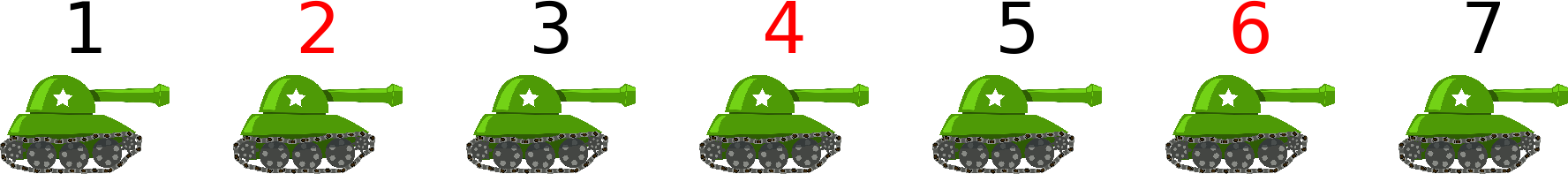
If the $k$ captured tanks are evenly spaced among the $n$ (sorted) total tanks, then the number of unobserved tanks between each captured tank is $m/k-1$. Consider $n=7$ and $k=3$ with captured tanks labeled red ($m=6$). Here, each captured tank is flanked by $6/3-1=1$ unobserved tank on each side.
The estimator $\hat{n}$ for the total number of tanks is unbiased. To illustrate, I ran 100,000 simulations of the dgp with $n=100$ and $k=5$ using the capture_tanks function, then used $\hat{n}$ above to estimate the number of tanks from the max serial number in each simulated outcome (and $k$). The distribution of the estimated number of tanks $\hat{n}$ among the simulations is shown below.
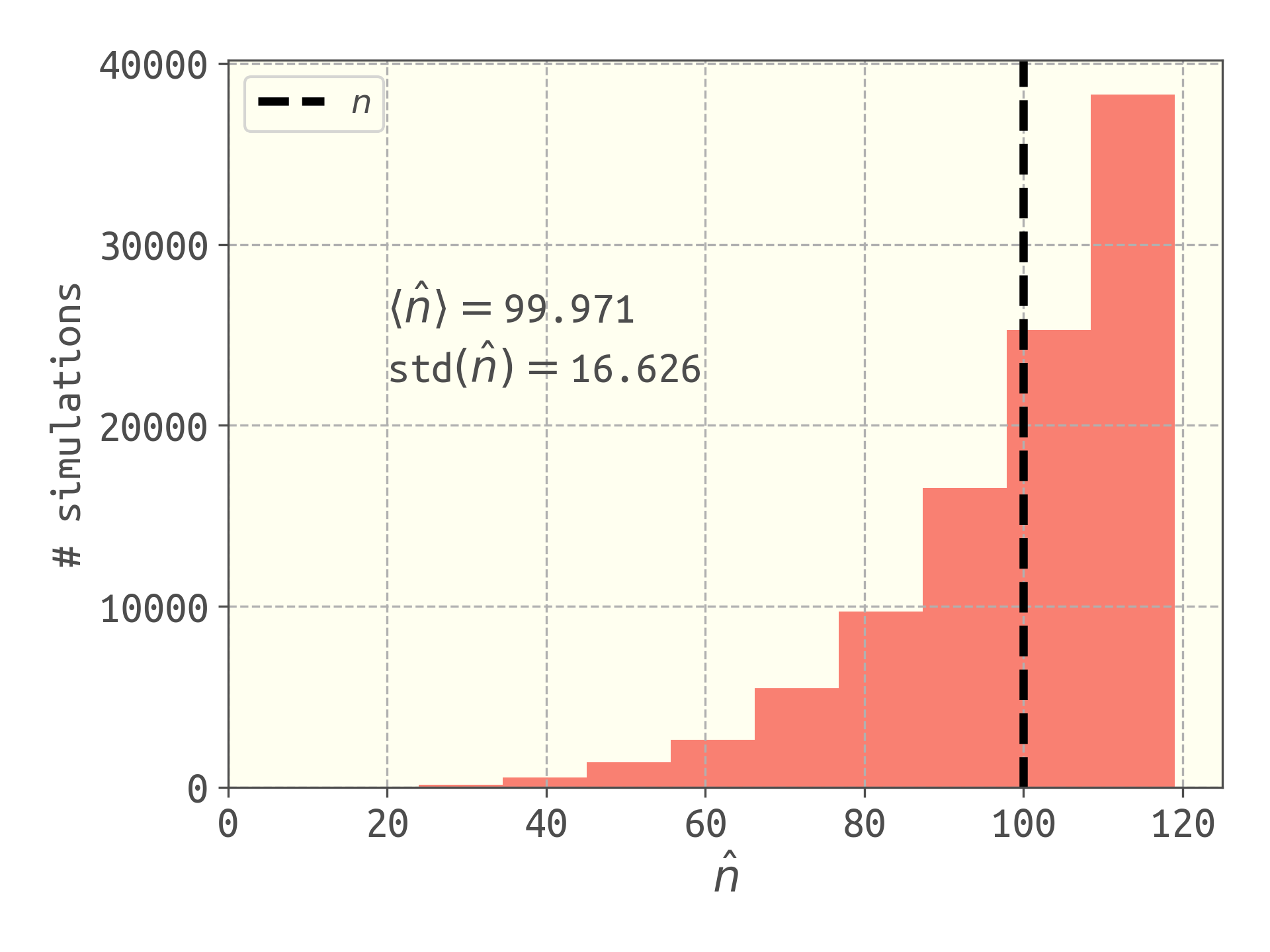
The estimator $\hat{n}$ is unbiased since, over many simulations, its average value is the true number of tanks.
One can also show that the estimator $\hat{n}$ is efficient [1], meaning that it exhibits the smallest variance among all other unbiased estimators.
Another desirable property of an estimator is consistency. Loosely, this means the distribution of the estimator $\hat{n}$ will concentrate on the true population size, $n$, as $k$ increases. That is, as we capture more tanks (increase $k$), the population estimate becomes more likely to be near the true population size. In the extreme case of $k=n$, we will always correctly estimate $n$. Below, I show the distribution of the estimated number of tanks $\hat{n}$ among 100,000 simulations ($n=100$) for several different values of $k$. Indeed, the distribution concentrates on the true number of tanks as $k$ increases, suggesting that this estimator is consistent. If we have more data, our estimate is likely to be better.
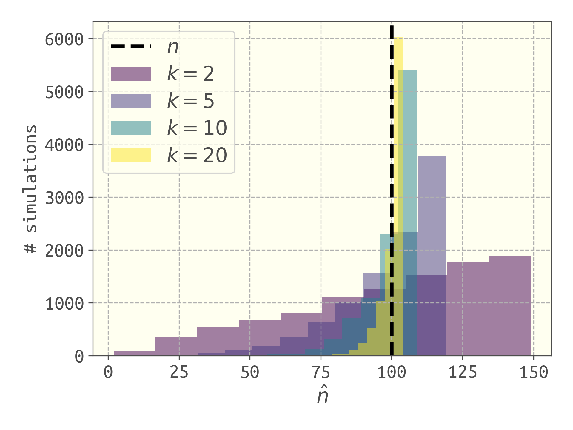
Computationally exploring the consistency of $\hat{n}$. The distribution of the estimated number of tanks concentrates on the true number of tanks as we capture more tanks.
confidence intervals
Our estimate $\hat{n}$ is a point estimate. In an interval estimate, we desire to estimate an interval in which the number of tanks belongs, which is associated with a confidence. The idea behind “confidence” is as follows. Say the maximum serial number we observed is $m=100$ with a sample size of $k=10$, and consider the hypothesis that the Germans have $10,000$ tanks. It could totally be true that we happened to capture only from within the first $100$ tanks of the $10,000$; we cannot disprove this hypothesis from our sample. However, given that $n=10,000$, it is an unlikely outcome that all $k=10$ tanks were sampled from only the first $100$ of the $10,000$ tanks; it is more likely to have a larger max serial number than $100$ if there were $10,000$ tanks. This gives us some confidence that the Germans have less than $10,000$ tanks.
Here is a computational and conceptually illustrative way to obtain a confidence interval for the number of tanks (using $k=10$, 200,000 simulations for each $n$). The solid line in the plot below shows the mean estimate of the number of tanks as a function of $n$. Because this is an unbiased estimator, this is a diagonal line with slope 1 and intercept 0. The green shaded band surrounding the mean excludes the bottom 5% and top 5% of the estimates. Now, imagine we observed $m=110$, giving the estimate shown as the horizontal dashed line. Our 90% confidence interval, based on these simulations, is shown as the purple bar on the $n$-axis. The lower bound is set at the lowest $n$ that would give us an estimate that high, excluding the top 5% of estimates. The upper bound is set at the highest $n$ that would give us an estimate this low, excluding the bottom 5% of estimates. For example, with $m=110$, we would reject the null hypothesis that $n>150$ at a level of significance of 5%, since it is sufficiently unlikely that the max serial number would be so low (110) if there were truly more than 150 tanks.
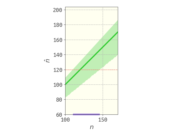
The estimate of $n$, $\hat{n}$, versus the true $n$. The green shaded band excludes the top 5% and bottom 5% of estimates. Here, $k=10$. The red, horizontal, dashed line shows the estimate for an observation $m=110$, and the purple band on the $n$-axis shows the confidence interval.
(update) A Bayesian treatment of the German tank problem
See my preprint “A Bayesian treatment of the German tank problem” on arXiv here.
references
[0] J. Champkin. The German tank problem. Great moments in statistics. https://rss.onlinelibrary.wiley.com/doi/pdf/10.1111/j.1740-9713.2013.00706.x <– fantastic overview
[1] Goodman LA. Serial number analysis. Journal of the American Statistical Association. 1952
[2] Ruggles R, Brodie H. An empirical approach to economic intelligence in World War II. Journal of the American Statistical Association. 1947
[3] KC Border’s Introduction to Probability and Statistics notes http://www.math.caltech.edu/~2016-17/2term/ma003/Notes/Lecture18.pdf
[4] Johnson RW. Estimating the size of a population. Teaching Statistics. 1994 <– gives nice intuitive arguments