dynamic models for liquid flow into/out of tanks with complicated geometries
author: Cory Simon
Problem setup
Liquid continuously flows into a truncated square pyramidal tank at a rate $q_i=q_i(t)$ [m$^3$/s]. Hydrostatic pressure drives flow out of the tank through a narrow pipe at its base; via Bernoulli’s equation, the outlet flow rate $q\propto \sqrt{h}$, where $h$ [m] is the liquid level in the tank.
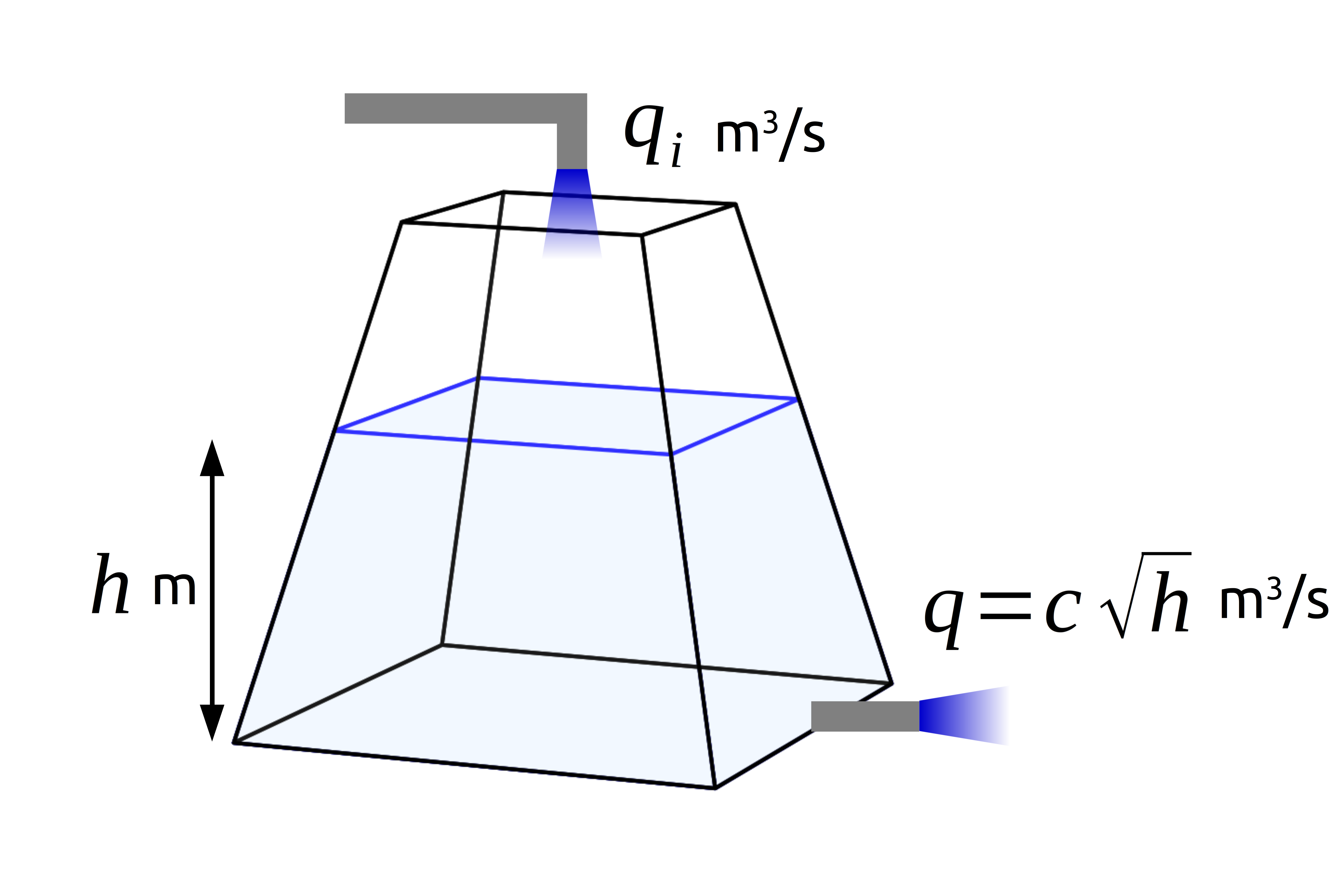
The goal here is to derive a dynamic model for the liquid level $h=h(t)$ given any input $q_i(t)$. The outlet flow rate then follows as $c\sqrt{h(t)}$. The proportionality constant $c$ is a characteristic of the liquid in the tank and the geometry of the exit line; it can be measured experimentally.
Mathematical model
Taking the liquid as incompressible, a mass balance (system boundary: the tank) implies a volume balance: $$\dfrac{dV}{dt}=q_i-c\sqrt{h}$$ where $V=V(t)$ is the volume of liquid in the tank at time $t$. This differential equation is intuitive if we multiply it by $dt$. Within a differential time window $dt$, we can view $q_i(t)$ and $h(t)$ as constant. In a differential time span $dt$: the amount of liquid that entered the tank is $q_idt$; the amount of liquid that exited the tank is $c\sqrt{h}dt$; the change in volume $dV$ of liquid in the tank within the differential time span $dt$ then must be $(q_i - c\sqrt{h})dt$.
The [agnostic to tank geometry] volume balance as written is not so helpful. It cannot be directly solved since $V$ is coupled to $h$ through the tank geometry, i.e., $V=V(h)$. Consider $q_i$ and $h$ known at a given moment. Then, the volume of liquid in the tank will change by $dV = (q_i - c\sqrt{h})dt$ after a differential time $dt$. But changing the volume will in turn change the liquid level $h$. So, to compute $dV$ at the next time step, we’d need to know how $h$ changed after we incremented the volume by $dV$ in the first step. This is where the tank geometry comes in.
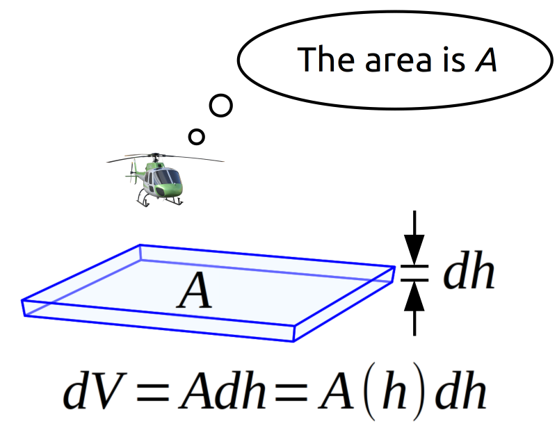
Consider when the liquid level changes by a differential length $dh$. This corresponds to adding a small slice of liquid whose volume is $dV$. We relate $dV$ and $dh$ through the area $A$ of the added slice of liquid from the helicopter view; $dV=Adh$ since, with such a thin slice, the areas of the bottom and top of the slice are the same. Generally, $A=A(h)$, as is the case for our tank geometry since the area from the helicopter view is larger for smaller liquid levels.
Therefore, a more helpful volume balance is: $A(h)\dfrac{dh}{dt}=q_i-c\sqrt{h}$ and is well-posed if we can find how the area from a helicopter view varies with $h$ in the tank geometry. This is the key to solving all tank problems of this nature, regardless of the tank geometry. We now impose our particular tank geometry to find $A(h)$ and complete the dynamic, differential equation model for $h(t)$.
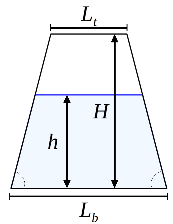
A little more about our truncated square pyramidal tank. The view from all four sides is equivalent and is below. Its height is $H$ [m]. The top and bottom base are of length $L_t$ and $L_b$ [m], respectively. All horizontal slices through the tank reveal a square cross-section. This is a right pyramid, meaning that its apex (if it weren’t truncated) is directly above the centroid of its base.
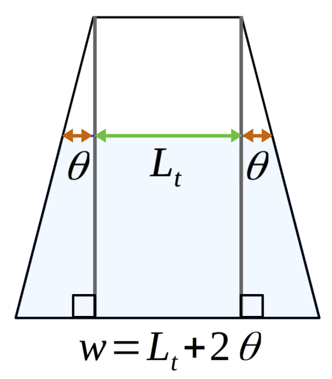
If we define $w=w(h)$ [m] to be the length of the line that the top of the liquid makes from a side view, then the area is simply $A(h)=[w(h)]^2$.
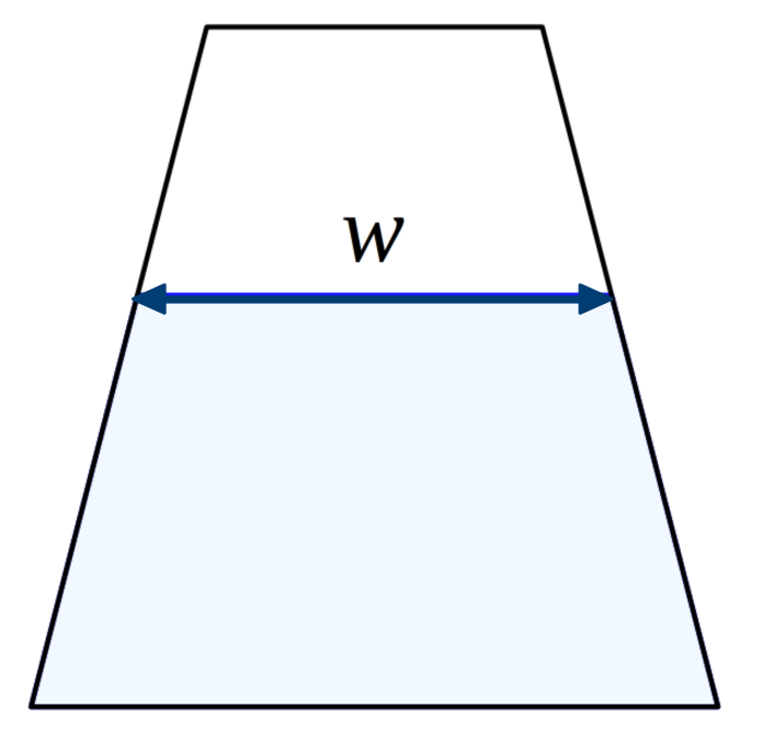
We can relate $w$ to the liquid level $h$, height of the tank $H$, and lengths of the bases $L_t$ and $L_b$ if we draw some right triangles. We bring in $L_t$ and write $w=L_t+2\theta$ with $\theta$ depicted below.
To determine $\theta$, we recognize two similar right triangles. At the bottom base, we decompose $L_b$ into $L_t$ plus $L_b-L_t$; half of the latter must be the base of the largest right triangle we drew. The smaller right triangle has a height of the tank $H$ minus that of the liquid $h$.
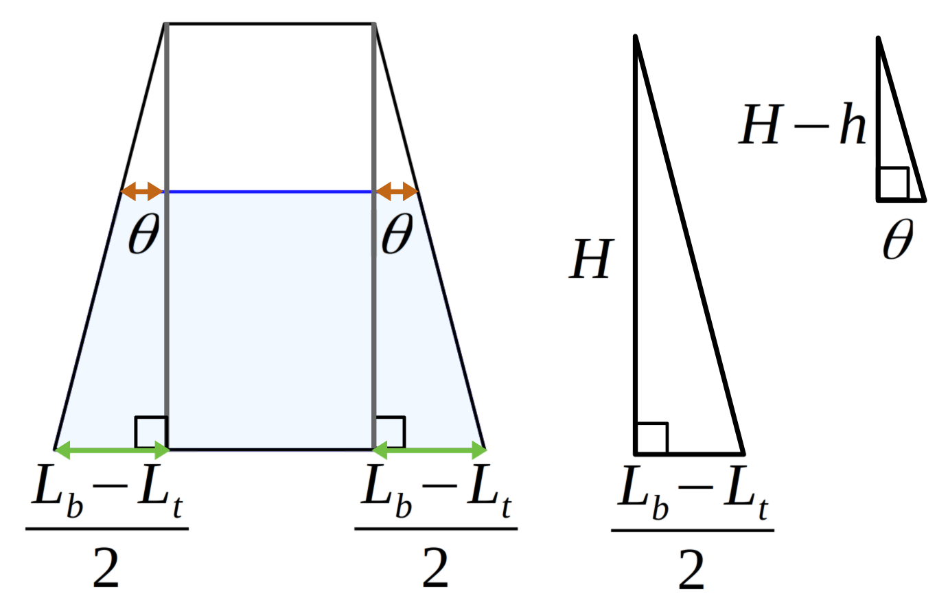
Because the triangles are similar, the ratio of the lengths of their two sides are equal: $$\dfrac{\theta}{H-h} = \dfrac{(L_b-L_t)/2}{H},$$ allowing us to solve for $\theta$ in terms of the geometric properties of the tank and the liquid level. Since the area is $A=(L_t + 2\theta)^2$, we arrive at: $$A(h) = \left[\frac{h}{H} L_t + \left(1-\frac{h}{H}\right)L_b \right]^2$$ The expression inside the brackets $[\cdot]^2$ is $w$. Intuitively, $w$ is a linear interpolation between $L_t$ and $L_b$. As $h\rightarrow 0$, $w$ approaches the bottom base height $L_b$. If $h \rightarrow H$, $w$ approaches the top base height $L_t$. [Some clever folks might write this expression directly, without the similar triangle argument.]
Finally, our expression $A(h)$ for the truncated square pyramidal tank completes the dynamic, differential equation model for the liquid level $h$ in the tank: $$\left[\frac{h}{H} L_t + \left(1-\frac{h}{H}\right)L_b \right]^2 \dfrac{dh}{dt}= q_i - c\sqrt{h}$$ This differential equation is non-linear. The solution $h(t)$ for a given initial condition $h(t=0)$ and input flow scheme $q_i(t)$ can be obtained numerically e.g. through OrdinaryDiffEq.jl.
Numerical solution
Let’s write code in Julia and use OrdinaryDiffEq.jl to numerically approximate the solution to our tank problem when the tank is initially empty ($h(t=0)=0$) and liquid flows into the tank at a constant rate.
First, we load some packages and define our parameters.
using OrdinaryDiffEq, CairoMakie

# specify tank geometry
H = 4.0  # tank height, m
Lb = 5.0 # bottom base length, m
Lt = 2.0 # top base length, m

# specify resistance to flow
c = 1.0  # awkward units

# inlet flow rate (constant)
qᵢ = 1.5 # m³/s

# initial liquid level
h₀ = 0.0
Second, we use OrdinaryDiffEq.jl to numerically solve the ODE.
tspan = (0.0, 155.0) # solve for 0 s to 150 s

# area from a helicopter view, m²
A(h) = (h/H * Lt + (1 - h/H) * Lb) ^ 2

# right-hand-side of ODE
rhs(h, _, t) = (qᵢ - c * sqrt(h)) / A(h)

# OrdinaryDiffEq.jl syntax
prob = ODEProblem(rhs, h₀, tspan)
h = solve(prob, Tsit5())
We next plot the solution.
ts = range(0.0, stop=152, length=300)
# easy as this to compute solution at an array of times!
hs = h.(ts)

fig = Figure()
ax  = Axis(fig[1, 1], xlabel="time, t [s]", ylabel="liquid level, h(t) [m]")
lines!(ts, hs, linewidth=4)
hlines!(H, linestyle=:dash)
xlims!(0, 151)
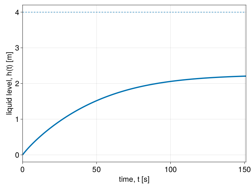
The plot above shows the resulting $h(t)$. The horizontal dashed line denotes the tank height $H$. Despite constant flow into the tank, the liquid does not overflow the tank since, if the tank is completely filled ($h=H$), hydrostatic pressure at the bottom drives flow out of the tank faster than the incoming flow rate $q_i$. The liquid level reaches a steady state $\bar{h}$ when the flow rate of liquid into the tank balances the rate at which hydrostatic pressure drives liquid out of the tank: $$q_i-c\sqrt{\bar{h}}=0$$ Here, with $q_i=1.5$ and $c=1$, the steady state liquid level is $\bar{h}$=2.25 m.