the orthogonal Procrustes problem
author: Cory Simon
The orthogonal Procrustes problem is to find the orthogonal matrix that maps a given set of points closest to another given set of points; the one-to-one correspondence of points between the two sets must be known a priori. The solution has applications in computer vision, molecular modeling, and speech translation.
The nomenclature refers to a character in Greek mythology, Procrustes, a bandit who stretched or cut off the limbs of his victims to fit his iron bed.
the set up
We have a set of $n$ points, $\mathcal{B}=\{\mathbf{b}_1, …, \mathbf{b}_n\}$, where $\mathbf{b}_i \in \mathbb{R}^d$.
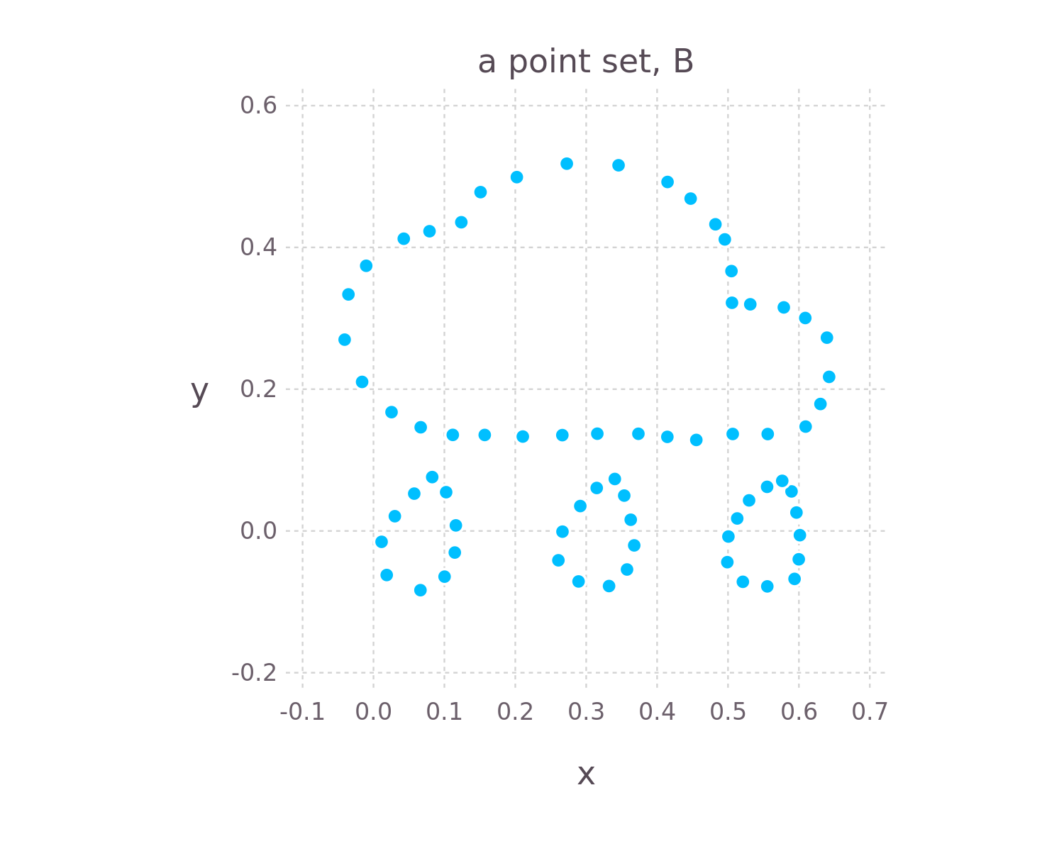
A set of $n$ points, $\mathcal{B}$. $d=2$ here for illustration.
A rogue troll rotated each point in $\mathcal{B}$ about the origin (using the same rotation matrix), then slightly perturbed its coordinates by adding Gaussian-distributed noise. This transformed set of points constitutes point set $\mathcal{A}=\{\mathbf{a}_1, …, \mathbf{a}_n\}$.
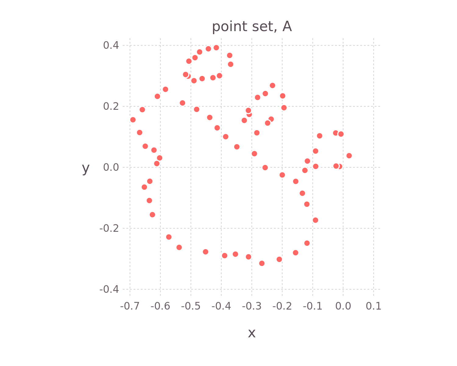
Point set $\mathcal{A}$ was obtained by rotating each point in the set $\mathcal{B}$ about the origin and adding independent, identically-distributed Gaussian noise to their coordinates.
The goal in the orthogonal Procrustes problem is to find the orthogonal matrix $R$ that maps the points in $\mathcal{A}$ to be the closest possible to the corresponding points in $\mathcal{B}$. Mathematically, the orthogonal Procrustes problem is: $$\DeclareMathOperator*{\argmin}{arg,min} R = \argmin_{\Omega : \text{ }\Omega ^T \Omega =I} \sum_{i=1}^n || \Omega \mathbf{a}_i - \mathbf{b}_i ||^2.$$ In words, we seek to minimize the sum of square distances between each vector $\mathbf{b}_i$ and the rotated vector $\Omega \mathbf{a}_i$ by choosing the $d$ by $d$ matrix $\Omega$ appropriately. The search here is not over all $d$ by $d$ matrices $\Omega$. There is a constraint that $\Omega$ must be an orthogonal matrix, i.e. $\Omega^T\Omega=I$; so the columns of $\Omega$ are unit vectors and are orthogonal to each other. This constraint ensures that transforming the points in $\mathcal{A}$ via left-multiplying by $\Omega$ does not change their norm (i.e. it is a rotation or reflection); note $||\Omega \mathbf{a}_i || ^ 2 =$ $(\Omega \mathbf{a}_i)^T (\Omega \mathbf{a}_i) $ $= \mathbf{a}_i^T \Omega ^T \Omega \mathbf{a}_i$ $= \mathbf{a}_i^T\mathbf{a}=||\mathbf{a_i}||^2$.
So the hope is that $R \mathbf{a}_i \approx \mathbf{b}_i$ for $i=1,…,n$.
Importantly, the one-to-one correspondences between the points in $\mathcal{A}$ with those in $\mathcal{B}$ are implicitly specified in the orthogonal Procrustes problem via the indexing of the points. That is, for each point in $\mathcal{B}$, we know which point in $\mathcal{A}$ is supposed to be mapped closeby via $\Omega$. So a clearer representation of the set up in the orthogonal Procrustes problem is below, where a gray line connecting two points indicates correspondence. Other, more sophisticated algorithms to align two point sets infer the correspondence between points automatically.
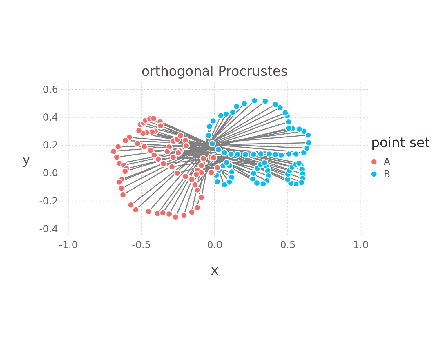
In the orthogonal Procrustes problem, we intend to map the $i$th point in $\mathcal{A}$ close to the $i$th point in $\mathcal{B}$. i.e. the hope is that $R\mathbf{a}_i \approx \mathbf{b}_i$, $\forall i$. This implicitly known correspondence between points is depicted by the gray lines connecting each $\mathbf{a}_i$ and $\mathbf{b}_i$ pair.
the analytical solution
First, we stack the points in $\mathcal{A}$ and $\mathcal{B}$ into matrices, $A$ and $B$, respectively, whose $i$th columns are $\mathbf{a}_i$ and $\mathbf{b}_i$, respectively. So $A := [\mathbf{a}_1 \cdots \mathbf{a}_n]$ and $B := [\mathbf{b}_1 \cdots \mathbf{b}_n]$.
Now we rewrite the objective in terms of the Frobenius norm $||\cdot ||_F$ of the matrix $\Omega A - B$. Generally, the Frobenius norm of a real matrix $Y$ (whose entries are by definition $y_{ij}$) is defined as $||Y||_F ^2:=\sum_i \sum_j y_{ij}^2$ and is equivalent to flattening the matrix, viewing it as a vector, and taking its L2 norm1. Since column $i$ of $\Omega A$ is $\Omega \mathbf{a}_i$, we can write the objective as: $$\DeclareMathOperator*{\argmin}{arg,min} R = \argmin_{\Omega :\text{ } \Omega ^T \Omega =I} || \Omega A - B ||_F^2.$$
By definition of the Frobenius norm, in terms of the components of matrices $\Omega A$ and $B$: \begin{align} R &= \argmin_{\Omega : \text{ } \Omega ^T\Omega =I} \sum_i \sum_j [(\Omega A - B)_{ij} ]^2 \\\ &= \argmin_{\Omega : \text{ } \Omega ^T \Omega =I} \sum_i \sum_j [(\Omega A)_{ij} - B_{ij} ]^2 \\\ &= \argmin_{\Omega : \text{ } \Omega ^T\Omega =I} \sum_i \sum_j [(\Omega A)_{ij}^2 + B_{ij}^2 -2 (\Omega A)_{ij} B_{ij}] \end{align} We recognize the sums of the two terms on the left of the right-most expression as $||\Omega A||_F ^2$ and $||B||_F ^2$, respectively: $$\DeclareMathOperator*{\argmin}{arg,min} R = \argmin_{\Omega : \text{ } \Omega ^T\Omega =I} { ||\Omega A||_F^2 + ||B||_F^2 + \sum_i \sum_j -2 (\Omega A)_{ij} B_{ij}}$$ We can simplify $||\Omega A||_F ^2$ since $\Omega$ is an orthogonal matrix. Recall the trace $\text{tr}(\cdot)$ of a matrix is the sum of its diagonal entries. Because entry $(i,i)$ of the matrix $Y^TY$ is $\mathbf{y}_i^T \mathbf{y}_i$, where $\mathbf{y}_i$ is column $i$ of the matrix $Y$, the square of the Frobenius norm of $Y$ is equal to the trace of $Y^TY$: $||Y||_F^2=\text{tr}(Y^TY)$. Since $\Omega$ is an orthogonal matrix: $$||\Omega A||_F^2=\text{tr}[(\Omega A)^T(\Omega A)]=\text{tr}(A^T \Omega^T \Omega A) = \text{tr}(A^TA) = ||A||_F^2$$
We made some progress by showing that the first two terms of the objective do not depend on $\Omega$, hence: $$\DeclareMathOperator*{\argmax}{arg,max} R = \argmax_{\Omega : \text{ } \Omega ^T\Omega =I} \sum_i \sum_j (\Omega A)_{ij} B_{ij}.$$ (Minimizing twice of a negative quantity is equivalent to maximizing the positive quantity.)
Now, via the definition of matrix multiplication, entry $(i, i)$ of $B^T \Omega A$ is the dot product of column $i$ of $\Omega A$ and row $i$ of $B^T$, which is column $i$ of $B$. Therefore2: $$\DeclareMathOperator*{\argmin}{arg,min} \DeclareMathOperator*{\argmax}{arg,max} R = \argmax_{\Omega : \text{ } \Omega^T\Omega=I} \text{tr}(B^T\Omega A)$$
Because the trace of a product of matrices is invariant to cyclic permutations of the matrix product: $$\DeclareMathOperator*{\argmin}{arg,min} \DeclareMathOperator*{\argmax}{arg,max} R = \argmax_{\Omega : \text{ } \Omega^T\Omega=I} \text{tr}(\Omega A B^T)$$
How to choose the orthogonal matrix $\Omega$ to maximize $\text{tr}(\Omega AB^T)$ is apparent after writing the $d$ by $d$ matrix $AB^T$ in terms of its singular value decomposition $AB^T=U\Sigma V^T$, where $U$ and $V$ are orthogonal matrices and $\Sigma$ is a diagonal matrix with [non-negative] singular values listed down its diagonal in a non-increasing manner. Then, we have: $$\DeclareMathOperator*{\argmin}{arg,min} \DeclareMathOperator*{\argmax}{arg,max} R = \argmax_{\Omega : \text{ }\Omega^T\Omega=I} { \text{tr}(\Omega U\Sigma V^T) = \text{tr}(V^T \Omega U \Sigma) }$$ The right equality follows from the invariance of the trace of matrix products to cyclic permutations of the product. Now, let $Z:=V^T \Omega U$, which is a product of orthogonal matrices; thus $Z$ is an orthogonal matrix itself (write out $Z^TZ$).
Finally, it becomes transparent of how to maximize $\text{tr}(Z\Sigma)$ because we are taking the trace of an orthogonal matrix times a diagonal matrix with entries arranged in a non-increasing order down the diagonal. Because $\Sigma$ is a diagonal matrix, $\text{tr}(Z\Sigma) = \text{tr}([\sigma_1 \mathbf{z}_1 \cdots \sigma_d \mathbf{z}_d])$, where $\sigma_i$ are the singular values of $AB^T$ that are across the diagonal of $\Sigma$. The $\mathbf{z}_i$’s are unit vectors since $Z$ is an orthogonal matrix, but cannot be chosen independently since they must be orthogonal to each other. Under this constraint, the trace of $Z\Sigma$ can be maximized by choosing $\Omega$ such that the $i$th entry of $\mathbf{z}_i$ is one and all other entries are zero. Under the constraint that the $\mathbf{z}_i$’s must be unit vectors and because $\sigma_1 \geq \cdots \geq \sigma_d \geq 0$, all other choices of $\mathbf{z}_i$ lead to a smaller number in the $(i, i)$th entry of $Z\Sigma$ and decrease the trace of $Z\Sigma$; of course, the $\mathbf{z}_i$’s under this choice are orthogonal.
So we choose $\Omega$ such that $Z$ is the identity matrix to maximize $\text{tr}(Z\Sigma)$. i.e., our solution is to choose $\Omega$ so that $Z=V^T\Omega U = I$. Right-multiply by $U^T$ and left-multiply by $V$, and, voila: $\Omega = VU^T$ maximizes $\text{tr}(Z\Sigma)$. Because $VU^T$ is a product of orthogonal matrices ($V$, $U^T$ orthogonality is constructed in the singular value decomposition), this choice of $\Omega$ satisfies our constraint that $\Omega^T\Omega=I$.
After all of this fancy matrix algebra, we find the optimal orthogonal matrix to transform the points in $\mathcal{A}$ so as to align them with the corresponding points in $\mathcal{B}$ by (i) computing the singular value composition of $AB^T=U\Sigma V^T$, then (ii) setting $R=VU^T$, then (iii) transforming each point in $\mathbf{a}_i \in \mathcal{A}$ via a matrix multiplication $R\mathbf{a}_i$.
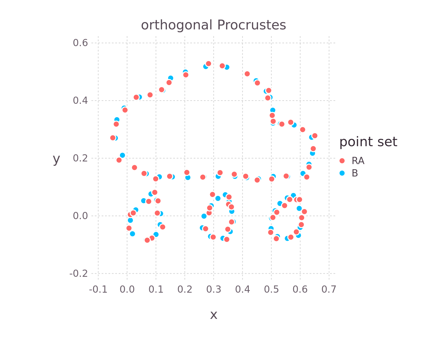
We computed the singular value decomposition of $AB^T=U\Sigma V^T$, then computed $R=VU^T$, then multiplied each point in $\mathcal{A}$ by $R$. Our solution to the orthogonal Procrustes problem nicely aligned the corresponding points!
numerical demonstration in Julia
Load in our point cloud (literally) of 70 points ($d=2$):
using DelimitedFiles
B = readdlm("point_cloud.txt") # 2 by 70 array
Rotate the point cloud about the origin by a known angle and add Gaussian noise to generate $A$:
rotation_matrix2d(θ::Float64) = [cos(θ) -sin(θ); sin(θ) cos(θ)]
θ = π * 0.8
R_known = rotation_matrix2d(θ)

ϵ = 0.01 # noise
A = R_known * B .+ ϵ * randn(size(B)...)
Compute the singular value decomposition of $AB^T$:
using LinearAlgebra

F = svd(A * B') # "F" for factorization
Recover the rotation matrix needed to transform the points in $A$ to re-align with those in $B$:
R = F.V * F.U' # orthogonal matrix
isapprox(R, rotation_matrix2d(-θ), rtol=0.01) # true

A_transformed = R * A # voila; pts in A aligned to those in B
See the Pluto.jl notebook here.
acknowledgement
Thanks to the group of Xiaoli Fern in Computer Science and my students Arni Sturluson and Carson Silsby at Oregon State University for the insightful discussion group we held on the orthogonal Procrustes problem. Also thanks to Wikipedia and these notes by John Mount.
footnotes
Since (i) the trace of a matrix is the sum of its eigenvalues and (ii) the eigenvalues of $Y^TY$ are the singular values of $Y$, also note that the Frobenius norm of a matrix is related to the sum of the squares of its singular values. ↩︎
We could also argue the term is $\text{tr}[(\Omega A)^T B]$ since entry $(i,i)$ of $(\Omega A)^T B$ is the dot product of column $i$ of B and row $i$ of $(\Omega A)^T$ which is column $i$ of $\Omega A$. We discovered that the trace of a matrix is invariant to transpose: $$\text{tr}(B^T\Omega A)=\text{tr}[(B^T(\Omega A))^T] = \text{tr}[(\Omega A)^T B]$$ This is sort of obvious in hindsight since transposing a matrix does not change its diagonal. ↩︎