Monte Carlo simulation of Buffon's Needle
authors: Arthur York, Cory Simon
Buffon’s Needle is a famous probability problem emanating from the 18th century.
setup
Imagine a floor marked with an infinite number of parallel, equidistant lines, a width $\ell$ apart.
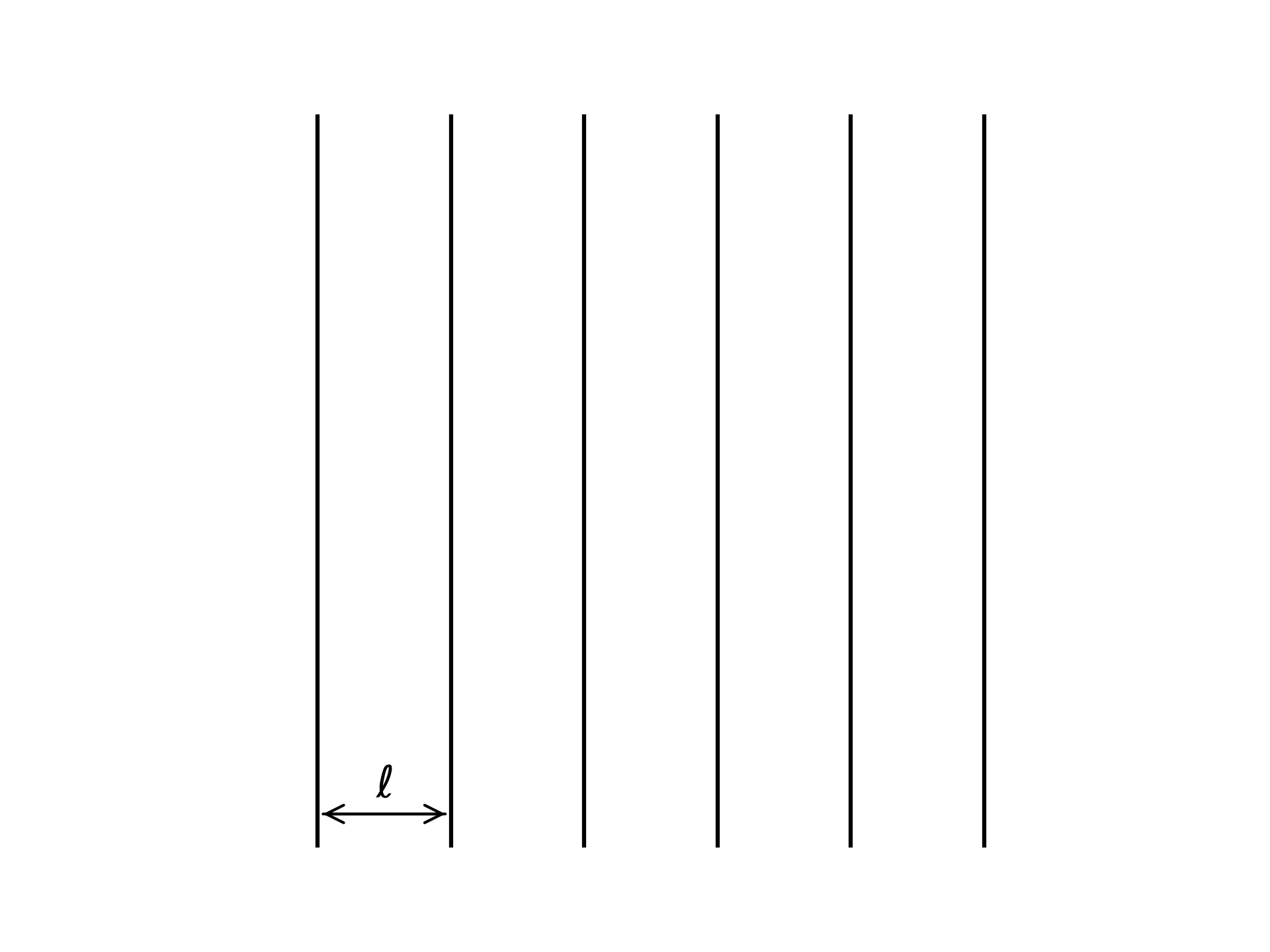
We now toss a needle of length $L<\ell$ onto the floor, where it lands at a uniform random position and with a uniform random orientation. Buffon’s needle problem is to determine the probability that the needle intersects one of the lines on the floor. The probability depends on the ratio of the length of the needle, $L$, to the distance between the lines on the floor, $\ell$.
this post
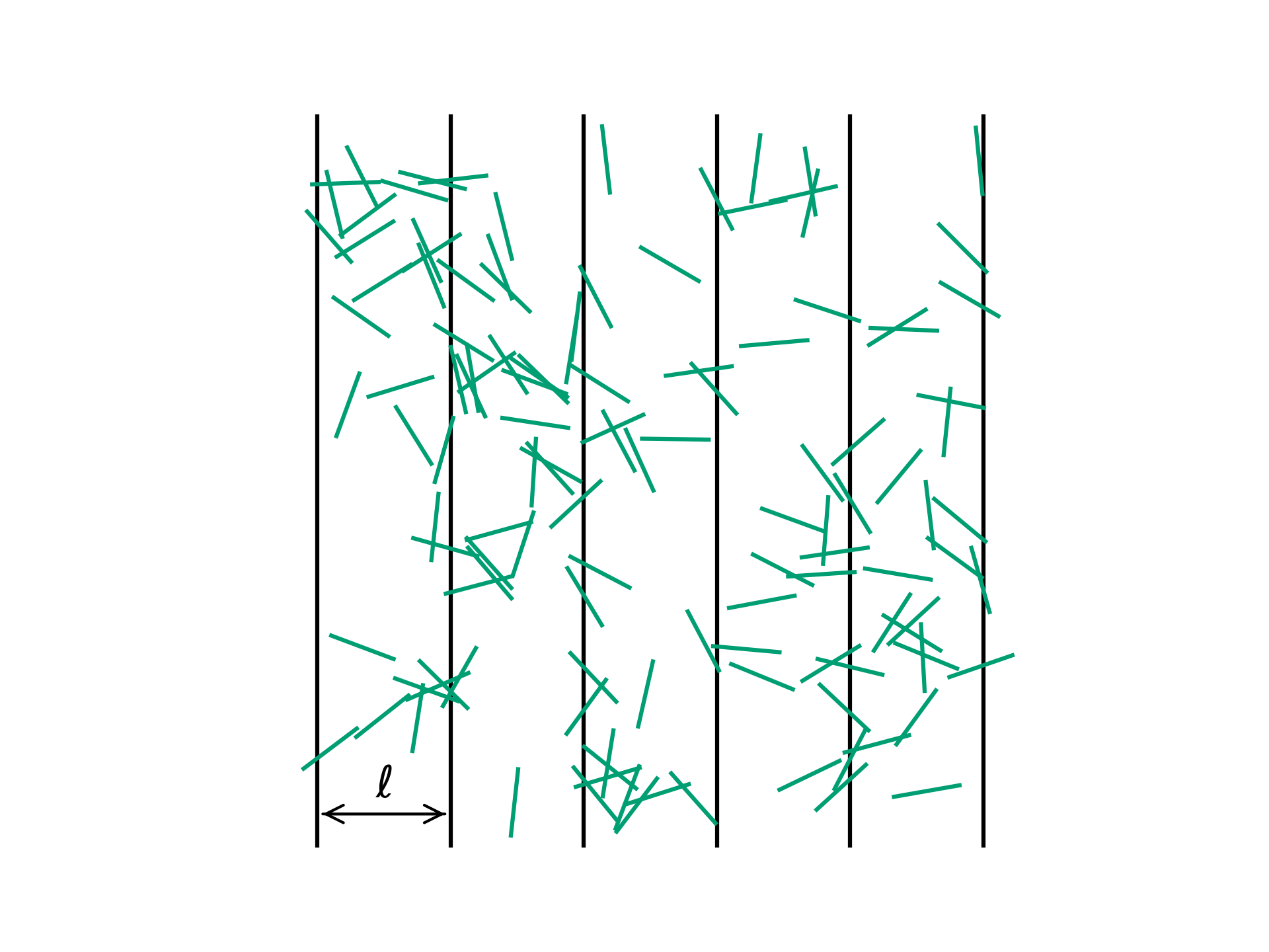
In this post, we conduct a Monte Carlo simulation of needle tossing in the Julia programming language to estimate the probability that a needle crosses a line. Below is an outcome from our simulation, where the needles are the teal-colored line segments. We also derive the analytical solution to Buffon’s needle problem to validate the simulations.
representing the floor
We create a data structure Floor to represent the floor, characterized by the distance $\ell$ between successive parallel lines, stretching in the $y$-direction and repeating ad infinitum in the $x$-direction.
struct Floor
    ℓ::Float64
end
representing a needle
The position and orientation of a needle on the floor is described by the Cartesian coordinates $(x,y)$ of its center and the angle $\theta$ it makes with the vertical axis.
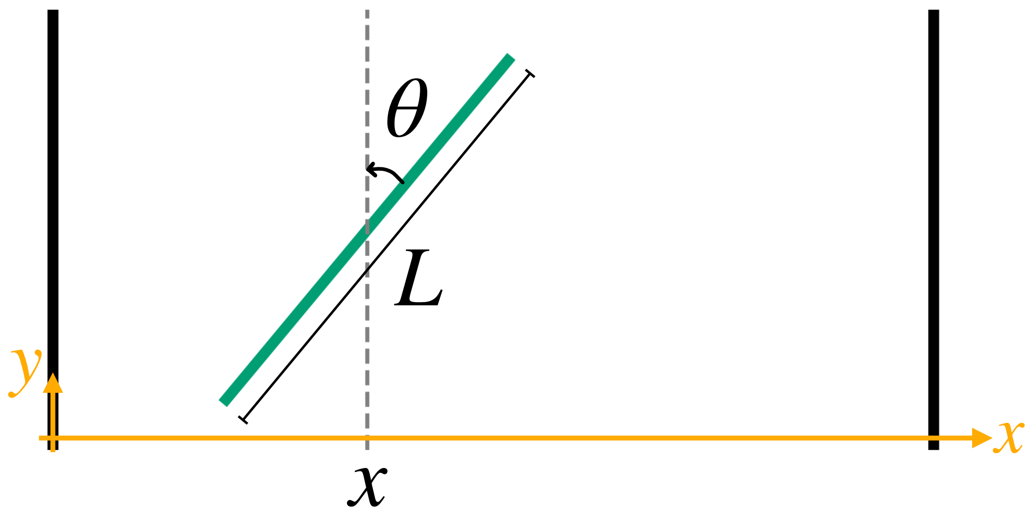
Note that the $y$ coordinate of a needle does not influence whether it intersects a line on the floor or not. Therefore, we do not need to consider it for our calculations; we only need to keep track of the $x$-coordinate and angle $\theta$ of a needle during the simulation.
We create a data structure Needle to represent a needle, storing its state $(x, \theta)$ and its attribute $L$.
struct Needle
    x::Float64
    θ::Float64
    L::Float64
end
the state space of a needle
Buffon’s needle problem concerns a needle being dropped anywhere on an infinite floor with repeating lines. But, it is impractical to create an infinite floor for the simulation. Instead, we only toss needles between two successive lines on the floor, i.e. $0 \leq x \leq \ell$. The estimate of the probability that the needle crosses a line is the same as for an infinite floor, owing to the symmetry of the floor.
It would be proper to allow the angle with the vertical $0 \leq \theta \leq 2\pi$, however we can take advantage of some rotational symmetry. A needle with angle $\theta$ appears equivalent to a needle with the same coordinates and angle of $\theta + \pi$. We therefore only allow $0 \leq \theta \leq \pi$ in our calculations.
The state space $\mathcal{R}$ of a needle is then: $$\mathcal{R} = \{ (x,\theta) \mid 0\leq x\leq \ell,0\leq \theta \leq \pi \}$$ Randomly throwing a needle on the floor in our simulation is equivalent to drawing a uniformly distributed sample from the state space $\mathcal{R}$.
simulation of needle tosses
For the simulation, we created a toss_needle function that returns a Needle uniformly distributed in the state space.
The function takes in as arguments the length of the needle, $L$, to toss, and the floor, floor, on which the needle is tossed.
function toss_needle(L::Float64, floor::Floor)
    x = rand() * floor.ℓ
    θ = rand() * π
    return Needle(x, θ, L)
end
This function essentially “samples” the needle state space, $\mathcal{R}$.
checking a needle for intersection with a line on the floor
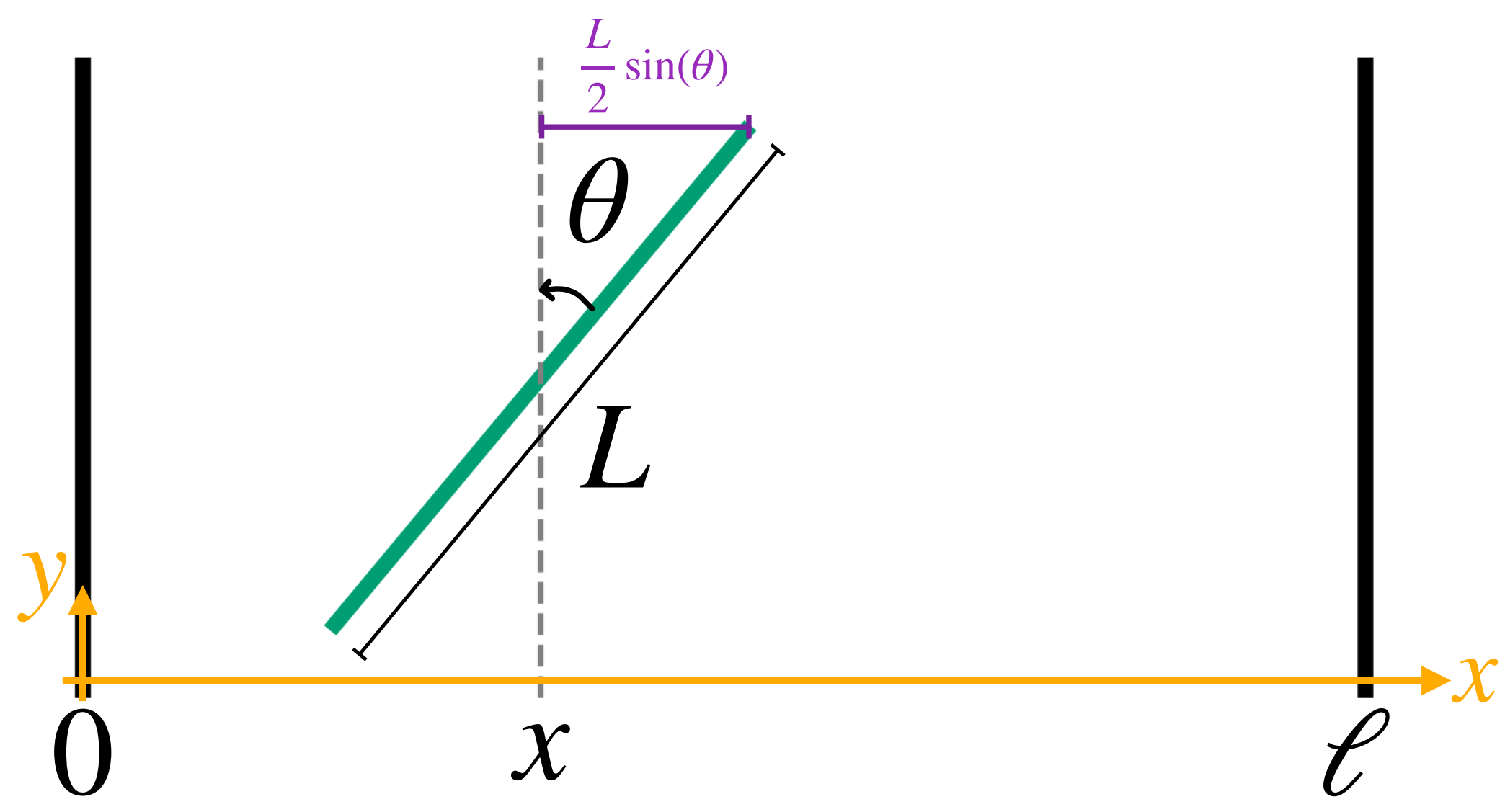
A needle will intersect a line if part of the needle overlaps $x=0$ or $x=\ell$. We check for overlap by checking the $x$-coordinates of the endpoints of the needles. If either the left or right endpoint of the needle is less than $0$ or greater than $\ell$, respectively, then the needle intersects a line.
The $x$-coordinates of the two endpoints of a needle are found as follows. Take the $x$-coordinate of the center of the needle. Then add and subtract half of the length of the projection of the needle onto the $x$-axis, $\frac{L}{2}\sin\theta$.
This generates two conditions for whether or not a needle crosses a line. A needle with coordinate $x$ and angle $\theta$ intersects a line if and only if:
The function cross_line takes a Needle and a Floor as arguments and returns true iff the needle intersects with a line on the floor.
function cross_line(needle::Needle, floor::Floor)
    x_right_tip = needle.x + needle.L / 2 * sin(needle.θ)
    x_left_tip  = needle.x - needle.L / 2 * sin(needle.θ)
    return x_right_tip > floor.ℓ || x_left_tip < 0.0
end
obtaining the probability analytically
To analytically obtain the probability of a needle intersecting a line, we can look at the fraction of the state space that leads to a needle intersecting a line. Below, we plot the state space $\mathcal{R}$ of the needle in the $(\theta, x)$ plane and shade it green and blue if that point in state space results in a needle not crossing or crossing a line on the floor, respectively. The blue regions, where the needle crosses a line on the floor, are described by $x+\frac{L}{2}\sin\theta>\ell$ and $x-\frac{L}{2}\sin\theta<0$. The total area of the blue regions divided by the total area of the state space is then the probability of a needle intersecting a line.
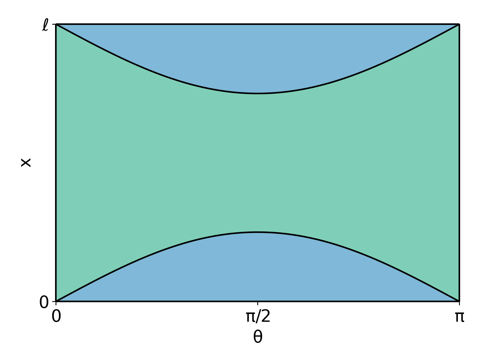
The area of the total state space of the needle is: $$A_T=\int_{0}^{\pi}\int_0^{\ell} dx d\theta=\ell\pi$$ The area of the state space satisfying $x-\frac{L}{2}\sin\theta\leq0$ is: $$A_1=\int_{0}^{\pi}\left(\frac{L}{2}\sin\theta\right)d\theta=L$$ The area of the state space satifying $x+\frac{L}{2}\sin\theta\geq \ell$ is: $$A_2=\int_{0}^{\pi}\ell d\theta-\int_{0}^{\pi}\left(\ell-\frac{L}{2}\sin\theta\right)d\theta=\int_{0}^{\pi}\left(\frac{L}{2}\sin\theta\right)d\theta=L$$ Therefore, the total area of needle state space that results in intersection with a line on the floor is: $$A_1+A_2=L+L=2L$$ and thus the probability of a needle landing on a line is the fraction of state space that is colored blue: $$\dfrac{A_1+A_2}{A_T}=\dfrac{2L}{\pi\ell}$$ Voila, the probability that a needle of length $L$ intersects a line on a floor with lines a distance $\ell$ apart is $2L/(\pi \ell)$. As $L /\ell$ decreases, the needle is short relative to the distance between the lines, and the probability of intersection decreases.
Intruigingly, this formula shows that one could compute the inverse of $\pi$ by throwing needles on a floor and counting the fraction that intersect a line, if $L=\ell/2$.
estimating the probability through a Monte Carlo simulation
We now estimate the probability that a tossed needle will cross a line on the floor with a Monte Carlo simulation.
We will toss a large number of needles on the floor with our function toss_needle and keep track of how many intersected a line on the floor, using our cross_line function.
Our estimate of the probability that a needle crosses a line on the floor is then the fraction of needles tossed that crossed a line, which we expect to be $2L/(\pi\ell)$.
function estimate_prob_needle_crosses_line(nb_tosses::Int,
                                           floor::Floor,
                                           L::Float64)
    nb_crosses = 0
    for t = 1:nb_tosses
        needle = toss_needle(L, floor)
        if cross_line(needle, floor)
            nb_crosses += 1
        end
    end
    # return fraction of needles that cross a line
    return nb_crosses / nb_tosses
end
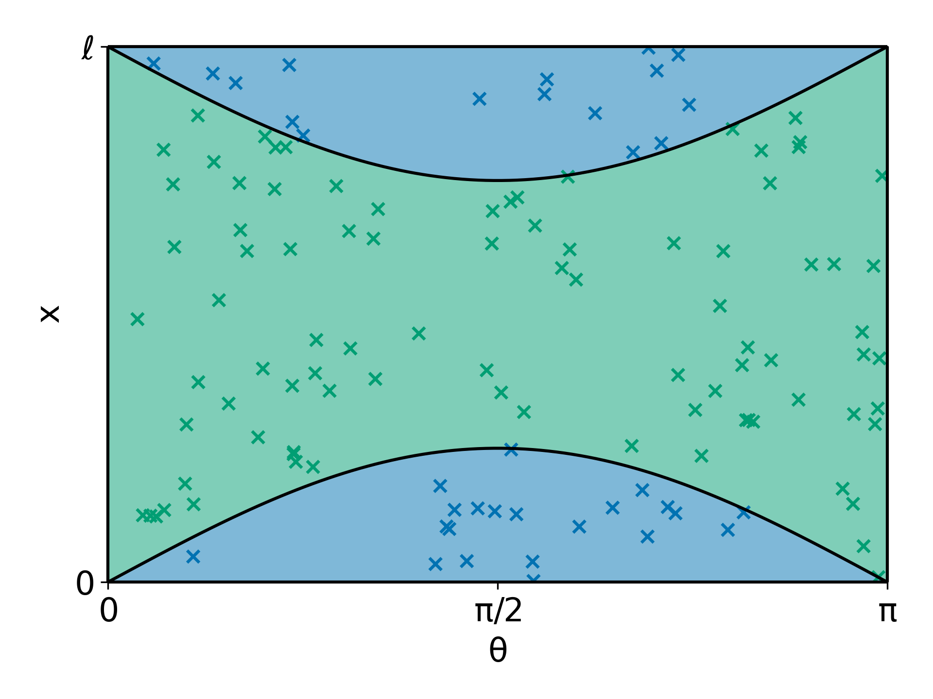
We plot randomly generated needles as points in their state space $\mathcal{R}$ below. The needles that were found to intersect a line on the floor are colored with blue. Those that didn’t intersect a line are colored green. The regions $x+\frac{L}{2}\sin\theta\geq \ell$ and $x-\frac{L}{2}\sin\theta\leq 0$ and their areas $A_2$ and $A_1$ from the analytical approach are shaded blue. Also note that if $\theta$ is close to zero or $\pi$, it is highly unlikely (less blue with $\theta$ fixed) that a needle will intersect a line because it is almost parallel with the lines on the floor. In contrast, fixed $\theta=\pi/2$ maximizes the probability that the needle intersects a line because then the needle is perpendicular to the lines on the floor.
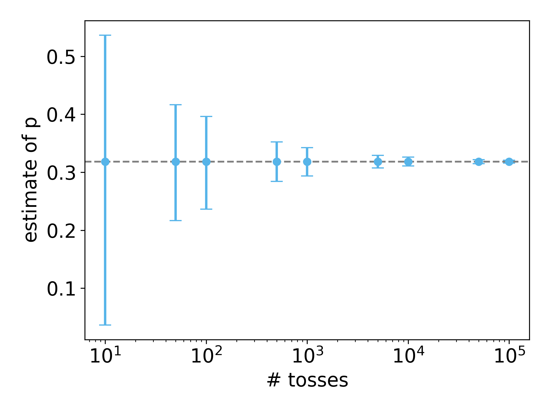
We compared the estimated probability from the Monte Carlo simulation to the theoretical probability $2L/(\pi \ell)$, and they are very close when the number of tosses used to estimate the probability is large. 👍
The plot below shows the estimated probability that a needle crosses a line– the fraction of needles that intersect a line in the Monte Carlo simulation– as we change the number of tosses used to make the estimate. Here, $\ell=2$ and $L=1$ so that the analytical solution is $\pi^{-1}$, shown as the horizontal, dashed line. The dots show the average estimation among 5,000 simulations for the fixed number of tosses, which agrees with the theoretical probability. The error bars include the middle 90% of the estimates. As we use more tosses to estimate the probability of intersection, the error bars shrink, meaning that the estimate exhibits less variance.
While Buffon’s needle is a toy problem, it illustrates many principles of Monte Carlo simulations used in statistical mechanics.
Finally, we point the reader to an extension of Buffon’s needle problem: Buffon’s noodle problem.