the freely jointed chain model
author: Cory Simon
Single-molecule force spectroscopy is a technique to gauge the binding forces within and mechanical properties of biopolymers. For example, consider a DNA unzipping experiment. At the end of a double-stranded DNA molecule, one strand is tethered to a fixed position, and the other, complementary strand is attached to a microsphere under an optical trap. Then, the two strands are pulled apart, and the force is measured as the hydrogen bonds between base pairs break and the DNA molecule unzips.
An intuitive observation is that a larger force is required to unzip GC-rich regions compared to AT-rich regions. This is consistent with the number of hydrogen bonds that hold together the base pairs: two in the case of A-T and three in the case of C-G. [ref] Dynamic DNA force spectroscopy can interrogate DNA-protein binding by measuring the force to disrupt the DNA-protein interaction as the DNA unzips [ref].
Physical models of biopolymers such as DNA are useful for interpreting and gleaning insights from DNA unzipping experiments. This blog post is the first in a series to explore such models. We begin by investigating a simple system: modeling a force spectroscopy experiment conducted on a single strand of DNA.
The freely jointed chain (FJC) model
The freely jointed chain (FJC) is a simplified structural model of a polymer such as single-stranded DNA. The FJC consists of $n$ rigid, linear monomers of length $b$, known as Kuhn segments. The $n$ monomers are joined together at their ends by freely rotating joints to form a chain. By allowing the joints to freely rotate, we neglect steric hindrance between any two given monomers (excluded volume) and allow all possible rotations between two consecutive monomers to be visited in an unbiased manner.
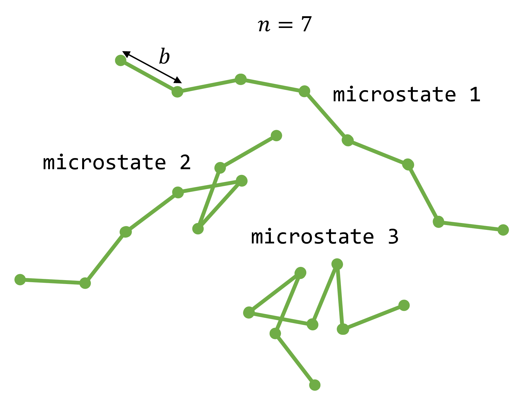
Fig. 1: Three examples of microstates that a freely jointed chain with $n=7$ monomers may adopt.
The freely jointed chain under an external pulling force
Now consider a FJC polymer in a force spectroscopy experiment. One end of the polymer is tethered to a fixed position. The other end is subject to a pulling force of magnitude $f$ with a direction to the right of the page. Let $x$ be the end-to-end distance of the polymer under this force $f$.
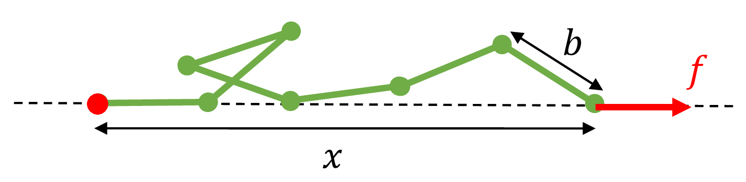
Fig. 2: A freely jointed chain subject to a pulling force $f$ to the right along the axis of the dashed line. The red ball on the left indicates that the left end of the polymer is tethered to that fixed position.
The question we will now address with statistical mechanics is: at equilibrium, what is the expected end-to-end distance $\langle x \rangle$ that the FJC polymer will adopt under this external force $f$?
From a purely mechanical perspective, one might incorrectly conclude that the force will induce the polymer to maximally extend until $x=nb$. The reasoning is as follows. The potential energy of the polymer, $-fx$, is minimized when it is fully extended. This is analogous to the potential energy of a soccer ball on a hill, $mgh$ ($m$: mass of soccer ball, $g$: gravitational acceleration, $h$: height of the ball). A soccer ball, under the external gravitational force of $mg$, will roll down the hill to its equilibrium position of lowest potential energy. Similarly, why wouldn’t the FJC polymer maximally extend under its external force $f$ to achieve its minimum energy position at equilibrium?
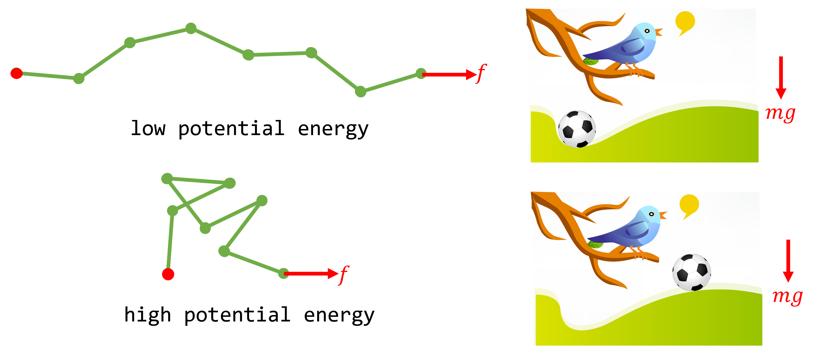
Fig. 3. When the polymer system is subject to the external force $f$, its potential energy is $-fx$. Shown are two example microstates of low and high potential energy and the analogy with a soccer ball on a hill subject to the gravitational force $mg$.
At molecular scales, we must also consider thermal fluctuations of the polymer and thus entropy. Entropy effectively gives rise to a second force in the opposite direction of $f$: when the polymer is fully extended ($x=nb$), there is only a single microstate that it can possibly adopt. On the other hand, when the polymer is half-extended, there are many microstates that the polymer can adopt that are consistent with $x=nb/2$. Therefore, from the perspective of maximizing entropy, full extension of the polymer imposes an entropic penalty. The average end-to-end distance $\langle x \rangle$ the polymer adopts is thus the classic story of competition between entropy and energy: the minimum potential energy configuration is full extension, but $x=nb$ corresponds to the $x$ with the minimal allowable microstates (one), hence lowest entropy.
The formula for the average end-to-end distance of a FJC polymer is: $$\frac{\langle x \rangle}{nb}= \coth(\beta bf) - \frac{1}{\beta b f},$$ where $\beta:=1/(k_B T)$. In the remainder of this post, we will use the principles of statistical mechanics to derive this formula.
The statistical mechanical ensemble
The appropriate thermodynamic ensemble to consider here is the isothermal-isoforce $nfT$-ensemble (analogous to the isothermal-isobaric ensemble): the temperature $T$, force $f$, and number of monomers $m$ are fixed in this polymer system. The partition function $\Delta(n, f, T)$ of the polymer system is a sum over all microstates $\nu$: $$\Delta = \sum_{\nu} e^{-\beta E_{\nu} + \beta f x_{\nu}}$$ where $E_{\nu}$ is the energy and $x_{\nu}$ is the end-to-end distance in microstate $\nu$. There are two ways to view this partition function. In the first way, we’re treating the polymer as ideal so that the potential energy $E_{\nu}=0$ for every microstate, and the $fx_{\nu}$ term plays the role of $PV_{\nu}$ in the isothermal-isobaric ensemble except with the opposite sign since, if $fdx$ is positive, work has been done $on$ the system. The other way to view the partition funciton $\Delta$ is as if the only energy associated with a microstate $\nu$ is the potential energy of the chain under the pulling force, which is $-fx_{\nu}$ as described above. i.e., $$\Delta =\sum_{\nu} e^{-\beta E_{\nu}} = \sum_{\nu} e^{\beta f x_{\nu}}$$ is an equally valid way to view the partition function.
Note that under the isothermal-isoforce ensemble, the probability of a microstate $\nu$, $p_{\nu}$, is proportional to the factor: $$p_{\nu} \sim e^{\beta f x_{\nu}},$$ rendering microstates with longer end-to-end distances $x_{\nu}$ as expontially more likely. However, as we will see, there are many more microstates associated with shorter chain lengths, so this is a classical competition between minimizing potential energy and maximizing entropy.
Characterizing the microstates
To perform the sum in the partition function, we first mathematically characterize a microstate of the polymer. For every monomer $i$, let $\vec{p}_i$ be the vector that traces it in the direction starting from the tethered monomer.
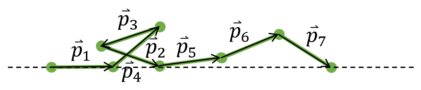
Fig. 4. We can draw the exact configuration of the polymer if given the vectors $\vec{p}_i$ that trace each monomer.
The angles that the vectors $\vec{p}_i$ take with respect to the axis determined by the force and tethering point, $\{\theta_i\}$, as well as the azimuthal angles $\{\phi_i\}$, are a more convenient description of the polymer’s microstate.
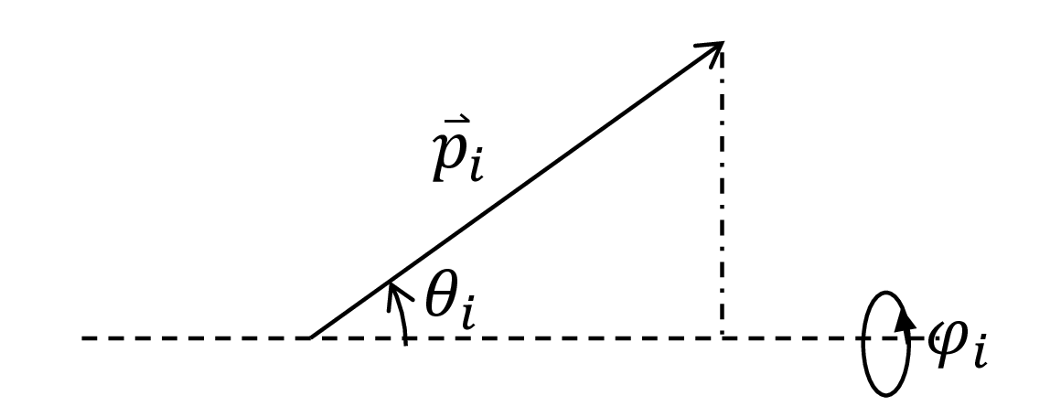
Fig. 5. The dashed line is the axis determined by the thethering point and the direction of the force. $\theta_i$ is the angle that the $i$th monomer takes with respect to this axis. $\phi_i$ is the azimuthal angle.
The angles $\theta_i \in [0, \pi]$ and $\phi_i \in [0, 2\pi]$. Thus, for the partition function, a sum over microstates is an integral: $$\sum_{\nu} = \int_0^{2\pi} \cdots \int_0^{2\pi} \int_0^{\pi} \cdots \int_0^{\pi} \sin \theta_1 \cdots \sin \theta_n d \theta_1 \cdots d \theta_n d \phi_1 \cdots d \phi_n.$$ The $\sin\theta_i$ terms arise from the surface element in spherical coordinates; without it, we would over-emphasize microstates towards the poles of the dashed axis.
We assumed here that the pulling force $f$ is always in the direction of $\sum \vec{p}_i - \vec{p}_1$. 1
Writing $x$ in terms of the microstate
We now write the end-to-end distance $x$ in terms of the microstate $\{(\theta_i, \phi_i) \}_{i=1,2,…,n}$. The drawing below shows that the extension of the polymer along the dashed axis due to monomer $i$ is given as $b \cos \theta_i$. Note that if $\theta_i> \pi / 2$, this quantity can be negative, indicating that the monomer is oriented such that the polymer is directed in the opposite direction of the force $f$.
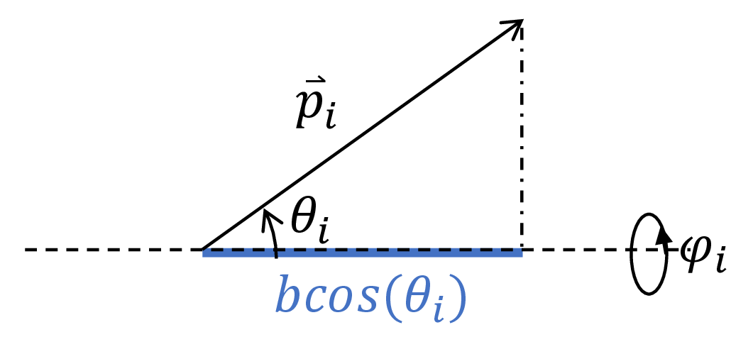
Fig. 6. Each monomer contributes $b \cos \theta_i$ to the end-to-end length of the polymer.
The total end-to-end distance is then the contribution due to each monomer: $$x(\theta_1, …, \theta_n, \phi_1, …, \phi_n) = \displaystyle \sum_{i=1}^n b \cos(\theta_i).$$
Writing the partition function
Using our expression for $x$, we now write the partition function $\Delta(n, f, T)$ as a nice product: $$\Delta(n, f, T)= \displaystyle\prod_{i=1}^n \int_0^{2\pi} \int_0^{\pi} \sin (\theta_i) e^{\beta f b\cos(\theta_i)} d \theta_i d \phi_i.$$ This gives: $$\Delta(n, f, T)= \left(4 \pi \frac{\sinh (\beta bf)}{\beta bf} \right)^n.$$
Calculating $\langle x \rangle$
The beauty of the partition function in statistical mechanics is that we can compute many properties of the system from its derivatives. The expected value of $x$ at equilibrium is, most generally: $$\langle x \rangle = \sum_{\nu} p_{\nu} x_{\nu},$$ where $p_{\nu}$ is the probability of observing microstate $\nu$ and $x_{\nu}$ is the end-to-end distance at that microstate. Given the statistical weight in the isothermal-isoforce ensemble (with $E_{\nu}=0$): $$p_{\nu}=\frac{e^{\beta f x_{\nu}}}{\Delta},$$ since the partition function is the normalization factor in the probability distribution governing the microstates. Plugging $p_{\nu}$ into the formula for $\langle x \rangle$ and recognizing this as a derivative of the partition function: $$\langle x \rangle = \sum_{\nu} \frac{e^{\beta f x_{\nu}}}{\Delta} x_{\nu}= \left(\frac{\partial \log \Delta}{\partial (\beta f)} \right)_{\beta,n}.$$
Upon taking the derivative, we get the Langevin function of $\beta b f$: $$\frac{\langle x \rangle}{nb} = \coth(\beta f b) - \frac{1}{\beta b f}.$$
Visualization
The figure below plots $\langle x \rangle / (nb)$ as a function of the non-dimensional quantity $\beta b f$. The result is intuitive. When the force is very large, the polymer becomes fully extended. When the temperature is very high, entropic effects dominate and the average end-to-end distance approaches zero. The result $\langle x \rangle \rightarrow 0$ as $\beta b f \rightarrow 0$ arises from symmetry: the polymer end is biased to the right ($x>0$) less and less by the force in this limit.
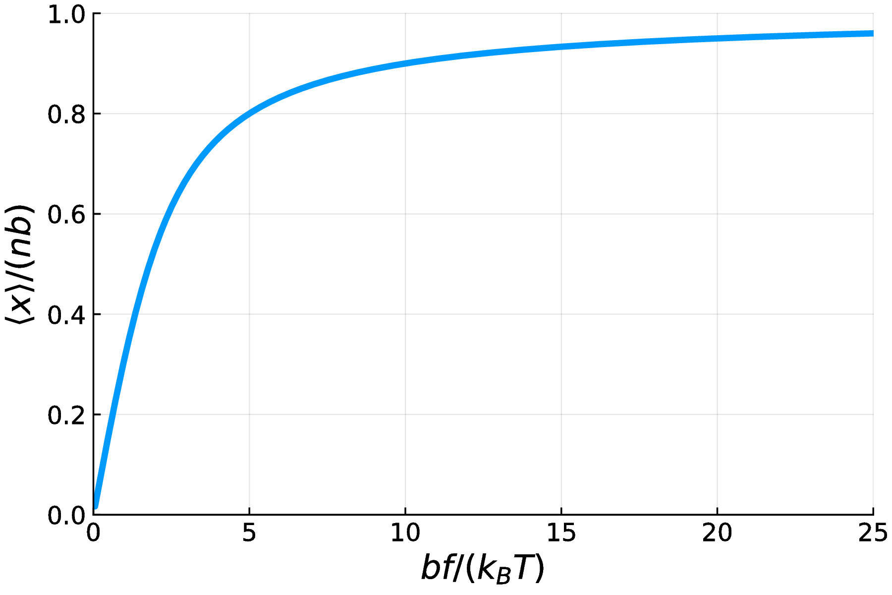
Fig. 7. A plot of the normalized expected end-to-end distance of a FJC polymer as a function of $\beta bf$. As the force $f$ increases, as the temperature $T$ decreases, and as the monomer length $b$ increases, the polymer becomes more fully extended.
Small force approximation
What happens when the force is small, such that $\beta b f « 1$? The Taylor expansion of the hyperbolic cotangent about zero is: $$\coth(\alpha) = \frac{1}{\alpha} + \frac{\alpha}{3} + \mathcal{O}(\alpha^3).$$
Thus, for small $f$: $$\langle x \rangle \sim \frac{\beta n b^2 f}{3}.$$ Solving for the force $f$, we get a form of Hooke’s Law: $$f = \frac{3}{\beta n b^2} \langle x \rangle.$$ This shows that the polymer behaves as an entropic spring. The spring constant reveals that a high temperature effectively renders the polymer more difficult to pull from $\langle x \rangle \sim 0$ due to larger entropic forces.
Large force approximation
When the force is large, such that $\beta bf » 1$, the hyperbolic cotangent term approaches unity. We then get: $$\langle x \rangle = nb \left(1 - \frac{1}{\beta bf}\right),$$ leading to a divergent force as the polymer approaches maximal extension: $$f= \frac{1}{\beta b} \frac{1}{1-\frac{\langle x\rangle}{nb}}.$$ That is, as the polymer approaches full extension, it gets progressively more difficult to pull it further.
Entropy as a function of $x$
If we tether both ends of the polymer to fixed positions in space, how does the entropy vary with $x$?
Method 1
The entropy is given by the Boltzmann equation: $$S(x)=k_B \log [\Omega(x)],$$ where $\Omega(x)$ is the number of microstates compatible with end-to-end length $x$. We can count such microstates using an integral with a delta function: $$\Omega(x)= \int_0^{2\pi} \cdots \int_0^{2\pi} \int_0^{\pi} \cdots \int_0^{\pi} \sin \theta_1 \cdots \sin \theta_n \delta \left(\sum_i b cos\theta_i - x \right) d \theta_1 \cdots d \theta_n d \phi_1 \cdots d \phi_n.$$ The delta function effectively sifts out the microstates that are compatible with an end-to-end distance $x$.
I’m not sure how to evaluate this integral. If you know, please email me or submit a pull request!
Method 2
Another approach is to apply the Gibbs formula for entropy: $$S = - k_B \sum_{\nu} p_{\nu} \log(p_{\nu}),$$ with: $$p_{\nu} = \frac{e^{\beta f x_{\nu}}}{\Delta}.$$ Here, $$\nu = (\theta_1, …, \theta_n, \phi_1, …, \phi_n)$$ as described above and the summation is actually an integral.
Method 3
Using Gibbs formula for entropy, we can show that the Gibbs free energy $G$ is: $$G = -k_B T \log \Delta.$$ From the first law of thermodynamics for reversible processes, $dG = -SdT - x df + \mu dn$, implying: $$-S = \left( \frac{\partial G}{\partial T} \right)_{f, n}.$$
Thus, in terms of the partition function $\Delta$: $$S = \frac{\partial}{\partial T} \left(k_B T \log \Delta\right)_{f, n}.$$
I think that owing to radially symmetry, the result will be the same if $f$ is only in the direction to the right of the page. On the other hand, the surface area of a sphere that $\sum \vec{p}_i$ can explore does get larger with increasing $x_{\nu}$… ↩︎